CHAPTER 19

FOUR SAMPLE FINAL EXAMINATIONS

These final examinations are actual exams held during the academic term, and each lasted 2 hours.

19.1 FINAL EXAM 1

Exercise 19.1

Assume that f(x) is absolutely integrable and a is a given real constant. Show that

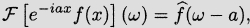
where is the Fourier transform of f.

Solution. Since |e^–iax| = 1 and f is absolutely integrable on (–∞, ∞), e ^{– iax}f(x) is also absolutely integrable on (–∞, ∞) and we have

for all ω∈

Exercise 19.2.

Hermite’s differential equation reads

(a) Multiply by e^–x2 and bring the differential equation into Sturm-Liouville form. Decide if the resulting Sturm-Liouville problem is regular or singular.

(b) Show that the Hermite polynomials

are eigenfunctions of the Sturm-Liouville problem and find the corresponding eigenvalues.

(c) Use an appropriate weight function and show that H₁ and H₂ are orthogonal on the interval (–∞,∞) with respect to this weight function.

Solution.

(a) Multiplying the differential equation by e^–x2 , we have

that is,

This is the self-adjoint form of Hermite’s equation, with p(x) = σ(x) = e^–x2 and q(x) = 0. Even though p, p^′, q, and σ are all continuous on the interval (– ∞, ∞), this Sturm-Liouville problem is singular since the interval is infinite.

(b) The Hermite polynomial of degree n is denoted by H_n(x).

• ForH₀(x)= 1 we have

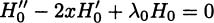
if and only if λ₀ = 0, and the eigenvalue corresponding to the eigenfunction H₀(x) is λ0 = 0.

• For H₁(x)=2xwe have

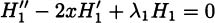
if and only if –4x + 2λ₁x = 0 for all x, that is, if and only if λ₁ = 2, and the eigenvalue corresponding to the eigenfunction H₁(x) is λ₁ = 2.

• For H₂{x)=4x² – 2 we have

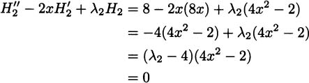
for all x if and only if λ₂ = 4, and the eigenvalue corresponding to the eigenfunction H/₂(x) is λ₂ = 4.

• For H₃(x)=8x³ – 12x we have

for all x if and only if λ₃ = 6, and the eigenvalue corresponding to the eigenfunction H₃(x) issλ₃ = 6.

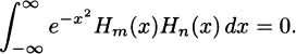
(c) There are two ways to answer this question. The more elegant method is as follows. We can show that the Hermite polynomials H_n, for n ≥ 0, are orthogonal on the interval (–∞,∞) with respect to the weight function r(x) = e^–x2 , by noting that

and subtracting, we have

Integration over the real line,we have

since the exponential kills off any polynomial as |x|→> ∞. Therefore, if m ≠ n, then

A more straightforward method is by integrating directly. For example,we note immediately that

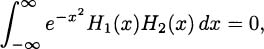
since the integrand is an odd function of x and we are integrating between symmetric limits.

Exercise 19.3.

Find all functionsϕ for which μ(x, t)= ϕ{x – ct) is a solution of the heat equation

where k and c are constants.

Solution. If ϕ is a twice continuously differentiable function such that

is a solution of the heat equation, then

and ϕ satisfies the equation

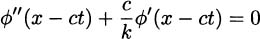
for all –∞ < x ∞ and t > 0; that is,

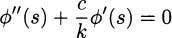
for all s ∈

Therefore, the solution is given by

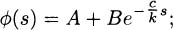
that is,

where A and B are arbitrary constants.

Exercise 19.4.

Consider the regular Sturm-Liouville problem

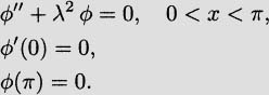
(a) Find the eigenvalues and the corresponding eigenfunctions ϕ_n for this problem.

(b) Show directly, by integration, that eigenfunctions corresponding to distinct eigenvalues are orthogonal.

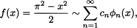
(c) Given the function f(x) = (π² – x²)/2, 0 < x < π, find the eigenfunction expansion for f.

(d) Show that

Solution.

(a) Case(i): λ = 0. The general solution to the equation ϕ″ + λ²ϕ = 0 in this case is

and differentiating,ϕ′(x)=c₁ and the condition ϕ′(0) = 0 implies that c₂ = 0. The condition 0(7r) = 0 implies that c₂ = 0, so there are no nontrivial solutions in this case.

Case(ii): λ ≠ 0. The general solution to the equation ϕ″ +λ²ϕ=0 in this case is

and differentiating, we get

The condition ϕ′(0) = 0 implies that c₂ λ = 0, so c₂ = 0. The solution is then

and the condition ϕ(π) = 0 implies that cos λπ = 0, and therefore the eigenvalues are

for n = 1,2,3,…. The corresponding eigenfunctions are

for n = 1,2,3,… .

(b) Letλ_n = (2n – l)/2 for n = 1,2,3,…. then for m ≠ n, we have

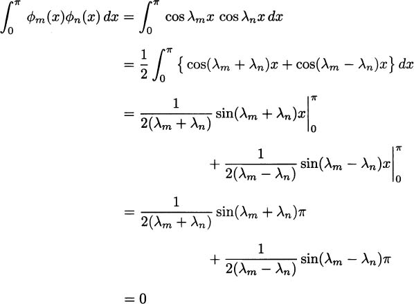
since (λ_m + λ_n)π = (m + n – 1)π and (λ_m – λ_n)π = (m – n)π. For n = m, we find

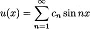
(c) Writing

the coefficients c_n in the eigenfunction expansionare found using the orthogonality of the eigenfunctions on [0,π] :

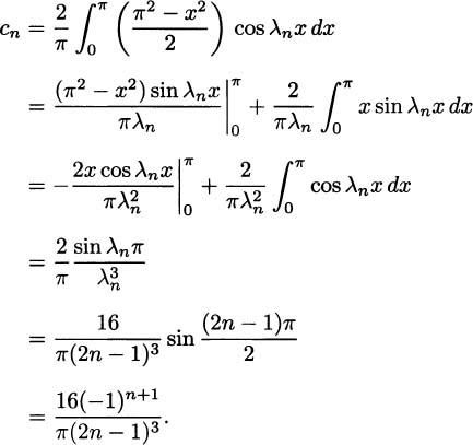
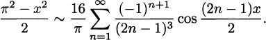
Therefore, the eigenfunction expansion of f is given by

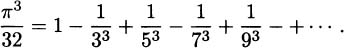
(d) In this particular problem, the eigenfunction expansion is actually the Fourier cosine series for f. Since the function F is piecewise smooth on the interval [0,π] and since the even extension of F to [–π, π] is continuous at x = 0, then by Dirichlet’s theorem the series converges to F(0) = π²/2 when x = 0, and therefore

Exercise 19.5.

Given the following boundary value-nitial value problem for the heat equation on [0,1]:

(a) Ifu(x, t) is the solution to this problem, find an initial boundary value problem satisfied by

(b) Solve the problem found in part (a) for w(x, t).

(c) Find the solution u(x, t) to the original problem.

(d) Find the time T₁ such that u(x, t) < 1 for every x ∈ [0,1] and every t > T₁.

Solution.

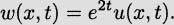
(a) If u(x,t) is the solution to the heat equation above and w(x, t) = e^2tu(x, t), then

so that

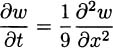
for 0 < x<1, t > 0. Therefore, w(x, t) = e^2tu(x, t) satisfies the boundary value-initial value problem

(b) Assuming a solution of the form w(x, t) = X (x).T(t) and separating variables, we get two ordinary differential equations,

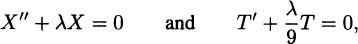
where λ is the separation constant.We can satisfy the two boundary conditions by requiring that X(0)=X(1)=0, so that X satifies the boundary value problem

The only nontrivial solutions occur when λ > 0, say λ = μ², where μ ≠ 0. In this case the general solution is

and from the boundary conditions, X(0) = 0 implies that A = 0, and since X(l) = 0, sin μ = 0. Thus, the eigenvalues are μ_n = nπ, with corresponding eigenfunctions X_n(x) = sinnπx for n ≥ 1. For n ≥ 1, the corresponding solution to

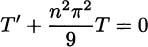
is T_n(t) = , and from the superposition principle, we write

for 0 < x < 1, t > 0. From the initial condition, we have

so that b_n = 0 for n ≠ 3, whileb₃ = 7. Therefore,

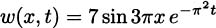
for 0 < x < 1, t > 0.

(c) The solution to the original problem is

for 0 <x < 1, t > 0.

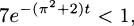
(d) Since

for all x ∈ [0,1] and all t ≥ 0, we can make u(x, t) < 1 by requiring that

and this will be true if that is,

that is,if

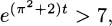
or equivalently,if

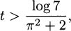
so we may take

19.2 FINAL EXAM 2

Exercise 19.6.

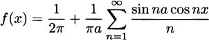
Let 0 < a < π; given the function

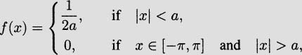
find the Fourier series for f and use Dirichlet’s convergence theorem to show that

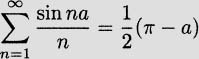
for 0 < a < π.

Solution. Since f(x) is an even function of the interval [–π,π], the Fourier series of f(x) is given by

where

and

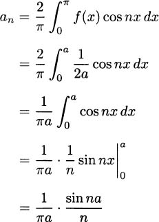
for n ≥ 1, and therefore

for –π<x < π

Since f(x) is continuous on the interval –a < x < a, the Fourier series converges to f(x) for – a < x < a; that is,

for –a < x < a. In particular, when x = 0, we have

so that

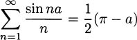
for 0 < a < π.

Exercise 19.7.

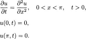
Consider the heat equation with a steady source

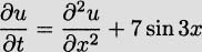
subject to the initial and boundary conditions

Solve this problem using the method of eigenfunction expansions. Show that the solution approaches a steady-state solution as t → ∞.

Solution. Since the problem already has homogeneous boundary conditions, we consider the corresponding homogeneous problem:

The eigenvalues and eigenfunctions for this problem are

for n ≥ 1. We write the solution to the nonhomogeneous problem as an expansion in terms of these eigenfunctions:

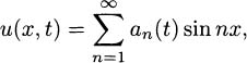
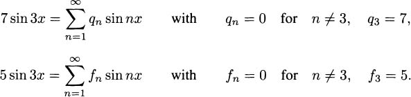
and determine the coefficients a_n (t) which force this to be a solution to the nonhomogeneous problem. We will need the eigenfunction expansions for Q(x) = 7sin3x and f(x) = 5 sin3x:

Substituting these expansions into the nonhomogeneous equation

we obtain

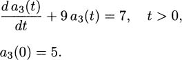
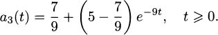
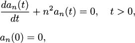
and the coefficient a₃(t) satisfiesthe initial value problem

The solution to this initial value problem is

that is,

Note that For n ≠ 3, we obtain

which implies that

for n ≠ 3. The solution to the heat equation with a steady source is therefore

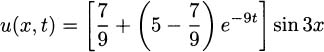
for 0≤ x ≤ π and t ≥ 0. For large values of t, this solution approaches r(x), where

for 0 ≤ x ≤ π. Differentiating this twice with respect to x, we see that

Since r(0) = r(π) =0, the function r(x) satisfies the boundary value problem

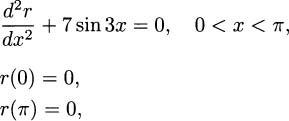
which is exactly the boundary value problem for the steady-state solution; that is, r(x) is the steady-state or equilibrium solution to the original heat flow problem.

Exercise 19.8.

(a) Using the method of characteristics, solve

(b) For which values of c does this initial value problem have a time-independent solution?

Solution.

(a) Let dx/dt = c; then along the characteristic curve x(t) = ct + a, where a = x(0), the partial differential equation becomes

so that

where K is a constant, and K = w(x(0), 0) – (l/2c)e^2x(t)+k so that

that is,

Given the point (x, t), let x = ct + a be the unique characteristic curve passing through this point; then

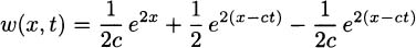
for –∞ < x < ∞ and t > 0.

(b) Note that if c = 1, the solution is

which is time independent.

Exercise 19.9.

Consider torsional oscillations of a homogeneous cylindrical shaft. If ω(x, t) is the angular displacement at time t of the cross section at x, then

where the initial conditions are

and the ends of the shaft are fixed elastically:

with α a positive constant.

(a) Why is it possible to use separation of variables to solve this problem ?

(b) Use separation of variables and show that one of the resulting problems is a regular Sturm-Liouville problem.

(c) Show that all of the eigenvalues of this regular Sturm-Liouville problem are positive.

Note: You do not need to solve the initial value problem, just answer the questions (a), (b), and (c).

Solution.

(a) Since the partial differential equation is linear and homogeneous and the boundary conditions are linear and homogeneous, we can use separation of variables.

(b) Assuming a solution of the form

and separating variables, we have two ordinary differential equations:

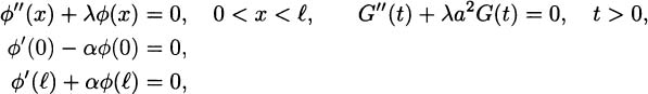
where the ϕ-problem is a regular Sturm-Liouville problem with

and

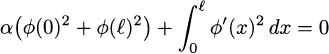
(c) We use the Rayleigh quotient to show that λ > 0 for all eigenvalues λ. Let λ be an eigenvalue of the Sturm-Liouville problem, and let ϕ(x) be the corresponding eigenfunction; then

and since q(x)= 0 for all 0 ≤ x ≤ .Note that if λ=0, then

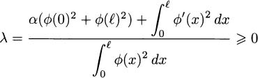
since p(x) = π(x) = 1 for 0 ≥ x ≥ ℓ. Note that if λ = 0, than

implies that

Since α > 0, this implies that ϕ(0) = 0 and ϕ() = 0, and since ϕ′ is continuous on [0, ], that ϕ′(x) = 0 for 0 ≤ x ≤ . Therefore, ϕ(x) is constant on [0, ]so that ϕ(x) = ϕ(0) = 0 for 0 ≤ x ≤ , and λ = 0 is not an eigenvalue. Thus, all of the eigenvalues λ of this Sturm-Liouville problem satisfy λ> 0.

19.3 FINAL EXAM 3

Exercise 19.10.

Assume that f″(t) is absolutely integrable and

Show that

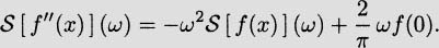
Solution. Assuming that lim_t→∞ f(t) = 0, and lim_t→∞f′(t) = 0, and integrating by parts, we have

We used the fact that

and

Exercise 19.11.

Legendre’s differential equation reads

(a) Write the differential equation in Sturm-Liouville form. Decide if the resulting Sturm-Liouville problem is regular or singular.

(b) Show that the first four Legendre polynomials,

are eigenfunctions of the Sturm-Liouville problem and find the corresponding eigenvalues.

(c) Use an appropriate weight function and show that P₁ and P_i are orthogonal on the interval (–1,1) with respect to this weight function.

Solution.

(a) Since

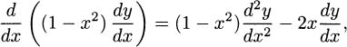
Legendre’s equation can be written as

(19.1)

which is the classical Sturm-Liouville form

with

for a <x <b where a = –1 and b = 1.

For a regular Sturm-Liouville problem we require the regularity conditions

are continuous on the closed interval a≤ x ≤ b, and

for a ≤ x ≤ b. We also require the boundary conditions

where at least one of α₁ and β₁ is nonzero and at least one of α₂ and β₂ is nonzero. Thus, it is clear that (19.1) is a singular Sturm-Liouville problem (no matter what the boundary conditions are) since one of the regularity conditions is violated, namely, p(–1) = p(1) = 0.

(b) • For P₀(x) = 1, we have

for –1 < x < 1, so that

is satisfied for λ = 0, and the eigenvalue corresponding to the eigenfunction p₀(x)=1 is λ₀= 0.

• For P₁ (x) = x, we have

for –1 < x < 1, so that

becomes

which is satisfied for λ = 2, and the eigenvalue corresponding to the eigen- function P₁ (x) = x is λ₁ =2.

• For P₂(x) = , we have

for – 1 < x < 1, so that

becomes

that is,

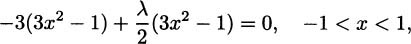
which is satisfied for λ = 6, and the eigenvalue corresponding to the eigenfunction P₂(x) = is λ₂ = 6.

• For P₃(x) = , we have

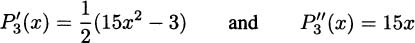
for –1 < x < 1, so that

becomes

that is,

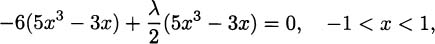
which is satisfied for λ = 12, and the eigenvalue corresponding to the eigenfunction P₃(x) = is λ₃ = 12.

(c) Using the weight function σ(x) = 1, for –1 < x < 1, we have

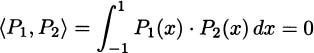
since the product P₁ (x)P₂ (x) is an odd function integrated between symmetric limits; thus, P₁ (x) and P₂(x) are orthogonal on the interval – 1 < x < 1 with respect to the weight function σ(x) = 1.

Exercise 19.12.

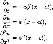
Find all functions ϕ for which u(x, t) = ϕ(x + ct) is a solution of the heat equation

where k and c are constants.

Solution. If u(x, t) = ϕ(x + ct) is a solution to the heat equation

let ξ = x + ct; then from the chain rule we have

Therefore, ϕ satisfies the ordinary differential equation

and the solution is given by

that is,

where A and B are arbitrary constants.

Exercise 19.13.

Let

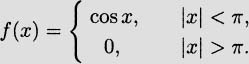
(a) Find the Fourier integral of f.

(b) For which values of x does the integral converge to f(x)

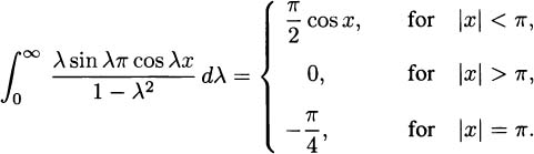
(c) Evaluate the integral

for –∞ < x < ∞.

Solution.

(a) The Fourier integral representation of f is given by

where

for λ ≥ 0. Since f(t) is an even function on the interval – ∞ < t <∞, then B(λ) = 0 for all λ ≥ 0, and

for all λ ^ 0.

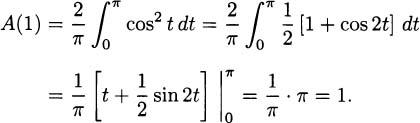
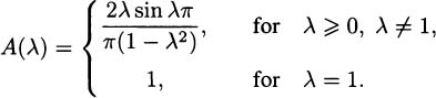
Now, for λ ≠ 1, we have

that is,

for λ ≥, λ≠.And for λ=1,we have

Therefore,

(b) Since f(x) is continuous for all x ≠ ±π, then from Dirichlet’s theorem, the Fourier integral representation converges to f(x) for all such x; that is,

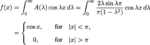
for all x ≠ ±π.

When x = ±π, from Dirichlet’s theorem the Fourier integral representation converges to

and

(c) From part (b) we have

19.4 FINAL EXAM 4

Exercise 19.14.

A fluid occupies the half-plane y > 0 and flows past (left to right, approximately) a plate located near the x-axis. If the x and y components of the velocity are

respectively, where U₀ is the constant free-stream velocity, then under certain assumptions, the equations of motion, continuity, and state can be reduced to

(19.2)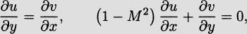

valid for all –∞ < x <∞, 0 < y < ∞. Suppose that there exists a function ϕ (called the velocity potential) such that

(a) State a condition under which the first equation in (19.2) becomes an identity.

(b) Show that the second equation in (19.2) becomes (assuming that the freestream Mach number M is a constant) a partial differential equation for ϕ which is elliptic if M < 1 or hyperbolic if M > 1.

Solution.

(a) If the velocity potential ϕ exists, then

and

and the mixed partial derivatives are equal at all points where they are continuous. Therefore, the first equation in (19.2) is an identity provided that

for all –∞ < x < ∞, 0 < y < ∞. Another possible solution is then obtained by assuming that the velocity potential ϕ(x, y) is twice continuously differentiable.

(b) Again, assuming the existence of a velocity potential, the second equation in (19.2) becomes

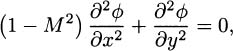
which is elliptic if 1 – M² > 0 and hyperbolic if 1 – M² < 0, that is, elliptic if M < 1 and hyperbolic if M > 1.

Exercise 19.15.

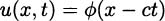
Besides linear equations, some nonlinear equations can also result in traveling wave solutions of the form

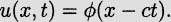
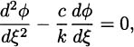
Fisher’s equation, which models the spread of an advantageous gene in a population, where u(x, t) is the density of the gene in the population at time t and location x, is given by

Show that Fisher’s equation has a solution of this form if ϕ satisfies the nonlinear ordinary differential equation

Solution. If u(x, t) = ϕ(x – ct), then

and Fisher’s equation becomes

for all x and t, so that if ϕ satisfies the nonlinear ordinary differential equation

then u(x, t) = ϕ(x – ct) is a traveling wave solution to Fisher’s equation.

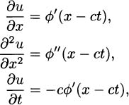
Exercise 19.16.

Given the regular Sturm-Liouville problem

(a) Find the eigenvalues and corresponding eigenfunctions ϕ_n(x) for this problem.

(b) Show directly, by integration, that eigenfunctions corresponding to distinct eigenvalues are orthogonal on the interval [0,π].

(c) Use the method of eigenfunction expansions to find the solution to the boundary value problem

(d) Solve the problem in (c) by direct integration and use this result to show that

for –π ≤ x ≤ π.

Solution.

(a) Since the parameter λ² ≥ 0, we need consider only two cases:

(i) If λ = 0, the differential equation is ϕ″ = 0 and has general solution ϕ(x) = Ax + B. The boundary condition ϕ(0) = 0 implies that B = 0, while the boundary condition ϕ(π) = 0 implies that A = 0, and there are no nontrivial solutions in this case.

(ii) If λ ≠ 0, the differential equation + ϕ″+λ²ϕ = 0 has general solution ϕ(x) = A cos λx + B sin λx. The boundary condition ϕ(0) = 0 implies that B = 0, while the boundary condition ϕ(π) = 0 implies that λπ = nπ for some positive integer n. Therefore, the eigenvalues and corresponding eigenfunctions are

for n ≥ 1.

(b) If m and n are distinct positive integers, then

and eigenfunctions corresponding to distinct eigenvalue are orthogonal.

(c) Let u(x) be a solution to the specified boundary value problem on the interval [0,π]. Expanding u(x) in terms of the eigenfunctions of the Sturm-Liouville problem, we have

for 0 ≤ x ≤ π. Differentiating this twice, we get

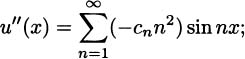
that is,

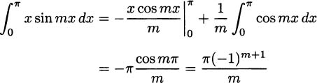
for 0 ≤ x ≤ π. Multiplying by sinmx and integrating, we have

From the orthogonality conditions, we find that

and

so that

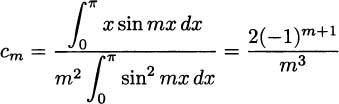
for m ≥ 1. Therefore,

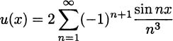
for 0 ≤ x ≤ π.

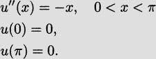
(d) The general solution to the differential equation u″(x) = –x is

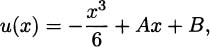
where A and B are constants. Applying the boundary conditions, u(0) = 0 implies that B = 0, while u(π) = 0implies that A = π²/6, and the solution is

for 0 ≤ x ≤ π. From part (c) we have

(19.3)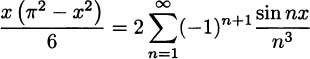

for 0 ≤ x ≤ π. The series on the right-hand side is the Fourier sine series for the odd function

on the interval [0,π], and since the odd extension is continuous on [–π, π], Dirichlet’s theorem says that (19.3) holds for all x with –π ≤ x ≤ π.

Exercise 19.17.

Find the solution to Laplace’s equation on the rectangle:

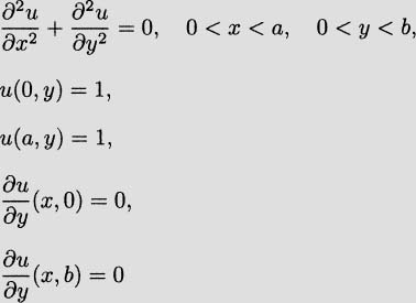
using the method of separation of variables. Is your solution what you expected?

Solution. Writing u(x, y) = X(x).Y(y), we obtain

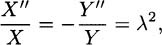
where λ is the separation constant, and hence we get the two ordinary differential equations

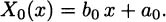
Solving the regular Sturm-Liouville problem for Y, for the eigenvalue = 0 the corresponding eigenfunction is

and the corresponding solution to the first equation is

For the eigenvalues = (nπ/b)², the corresponding eigenfunctions are

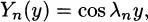
and the corresponding solutions to the first equation are

for n = 1,2,3, … Using the superposition principle, we write

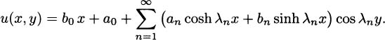
From the boundary condition u(0, y) = 1, we have

so that

while

for n = 1,2,3, From the boundary condition u(a, y) = 1, we have

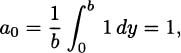
and integrating this equation from 0 to b we get b₀ a b = 0, and therefore b₀ = 0, so that

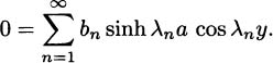
To evaluate the b_n’s, we multiply this equation by cos(mπ/b)y and integrate from 0 to b, to obtain b_m sinh(mπ/b)a = 0; that is, b_m = 0 for m= 1,2,3…. Therefore, the solution is u(x, y) = 1, which is not totally unexpected. The solution is unique and it is clear from the statement of the problem that u(x, y) = 1 satisfies Laplace’s equation on the rectangle and also satisfies all of the boundary conditions.

Exercise 19.18.

Solve the following initial value problem for the damped wave equation:

Hint: Do not use separation of variables; instead, solve the boundary value-i-initial value problem satisfied by w(x, t) = e^t . u(x, t).

Solution. Note that u(x, t) = e ^–t . w(x, t), so that

and

so

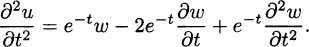
therefore,

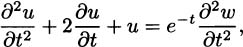
so that

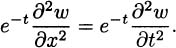
thus,if u is a solution to the original partial differential equation,since e^–t≠0,wsatisfies the initial value problem

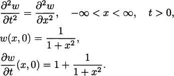
from d’Alembert’s soulation to the wave equation,we have(since c=1)

so that

for –∞<X<∞,t>0