In the last chapter, we covered myriad ways to take your data and load it into your BigQuery data warehouse. Another significant way of getting your data into BigQuery is to stream it. In this chapter, we will cover the pros and cons of streaming data, when you might want to use it, and how to do it.
Streaming bears little resemblance to loading. Most notably, there’s no way to activate it using the UI in the BigQuery console. Consequently, we’ll be using Python for our examples. In practice, you could run this code inside a Google Compute Engine (GCE) or Google Cloud Function. You might also run this code at the end of a processing pipeline you already have in your current architecture. Or you might add BigQuery as a streaming destination for data in addition to other sinks.
Also, the streaming methodology we’re discussing here is not Google Dataflow. Dataflow is another Google service that integrates closely with BigQuery, as well as external systems, Pub/Sub, Cloud Functions, and so on. Dataflow is capable of both streaming and batching incoming data. However, it has a different origin and requires a completely separate set of concepts and services. It definitely warrants a treatment of its own, which we’ll get to in the next chapter.
Another important note: BigQuery streaming is not available on the free tier of Google Cloud Platform. Most services have a threshold under which Google will not charge you, and in fact if you stay on the free tier, you may never even provide billing information. BigQuery streaming has no such threshold. To enable it, you must provide your billing information. The cost for the test data we’re messing with will not be high (at this writing, streaming costs a nickel per gigabyte), but it’s something to be aware of.
With all that out of the way, let’s dive in.
Benefits and Drawbacks
With loading, you have to wait until the job completes for your data to be accessible. You gain access to streamed data very quickly. This makes it ideal for scenarios where you want to query the data as soon as possible. These are things like click streams, user event tracking, logging, or telemetry. This is the signature and primary benefit of streaming. Data becomes available to query within a few seconds of the stream beginning to insert. You can begin to aggregate it, transform it, or pass it to your machine learning models for analysis. In high-traffic scenarios, this can give you rapid insight into what is happening with your business and application.
For example, let’s say you run an application with a fleet of mobile users. Each event a user performs on the application is streamed to BigQuery, and your analysis runs on the aggregate across users. Suddenly, after a code deploy, the rate for one of your events drops precipitously. This would give you a clue that there might be an undetected error occurring that is preventing users from reaching that page.
There are also great use cases for adaptive learning algorithms. For an ecommerce site, you might log an event every time a customer looks at a product, adds it to a cart, and so on. If you are streaming all of those events as they happen, you can monitor changes in sales trends as they occur. If you also store the referring URL for a given product view, you would know within minutes if a high-traffic site linked to yours and could adapt to present that new audience with other product opportunities. This could even all happen automatically at 3 AM while you were sleeping. (Of course, if these views were resulting in sales, you might want an alert to wake you up in this situation…)
I’m focusing on aggregations, trends, and speed because the trade-offs you make to get these benefits are not insignificant. Streaming is most appropriate for those situations because of the deficiencies.
Many of these scenarios would also be applicable for a Dataflow pipeline. Dataflow also requires a fair amount of code and tends to be more expensive than streaming. Once you have a solid grasp on loading, streaming, and Dataflow, you’ll be able to decide which of your use cases fit best with each technology. In reality, your business will have many use cases: the double-edged sword of being the data architect is that you get to (have to) understand all of them.
There are a few additional considerations around streaming.
Data Consistency
There is no guarantee with streaming that your event will arrive or that it will arrive only once. Errors in your application or in BigQuery itself can cause inserts to fail to arrive or to arrive several times.
Google’s approach to this is to request a field called insertId for each row. This field is used to identify duplicate rows if you attempt to insert the same data (or an insert is replayed) twice. The specifications say that BigQuery will hold onto a given insertId for “at least” one minute. If a stream errors and the state of your inserts is unknown, you can run the inserts again with the same insertIds, and BigQuery will attempt to automatically remove the duplicates. Unfortunately, the amount of time BigQuery actually remembers the insertId is undefined. If you implement an exponential backoff strategy for retrying after error, cap it under 60 seconds to be safe.
Even insertId comes with a trade-off though: the processing quotas are much lower if you are supplying insertId. Without insertId, BigQuery allows a million rows a second to be inserted. With insertId, that number drops to 100,000 per second. Still, 100,000 rows a second is nothing to scoff at. Even with thousands of concurrent users generating several events a second, you’d still be within quota. (The non-insertId, 1,000,000 rows/second quota is currently available only in beta.)
In scenarios where you are looking at data aggregation and identifying patterns, a few lost or extra events are no big deal. In a scenario that requires transactional guarantees, streaming is not an appropriate choice. Google provides guidance for querying and deduplicating rows after your stream has finished, so if you just need the guarantee later, that might be sufficient.
For the record, I have not often seen streaming either drop events or duplicate them, but that’s not a guarantee on which I’d want to base the integrity of my business’s data. (Side note: Google Dataflow implements insertId automatically and thus can guarantee “exactly-once” processing.)
Data Availability
As mentioned previously, data streamed to BigQuery becomes available in a few seconds. However, the data does not become available for copy or export until up to 90 minutes. You can’t implement your own aggregation windows by running a process every minute to grab all the new streamed data, dedupe it, and push it elsewhere.
There will be a column in your streamed table called _PARTITIONTIME which will be NULL when the data is not available for export/copy. You can use this to set up behaviors that do aggregate and additionally transform the data, but those pipelines may take a while to run.
Google does not specify what determines the delay for data insert or availability, but it is likely a factor of adjacent traffic, latency between GCP data centers, and the amount of free I/O available to the data center(s) your stream is executing on. They do say that “Data can flow through machines outside the dataset's location while BigQuery processes…” and that you will incur additional latency if you’re loading to a dataset from a different location.
When to Stream
Very high volume (thousands of events per second).
No need for transactionality.
Data is more useful in aggregate than by individual row.
You need to query it in near real time.
You can live with occasional duplicated or missing data.
Cost sensitivity is not a major issue.
You may be thinking that these are a lot of constraints for the benefit of immediate analytics. That’s true. Dealing effectively with data at such high velocity comes with trade-offs. With infinite budget and resources, a careful decision wouldn’t be required. Ultimately this decision will be based on whether the benefits outweigh the costs, both in money and in time.
Writing a Streaming Insert
In order to write an insert, we’ll have to put our code somewhere. You can run this code from your local machine or on the cloud shell. You can run it from there as well, or you can deploy it to Google App Engine.
Google App Engine
Google App Engine (GAE) is a great place to easily write code and deploy it with minimal configuration and no server management. Google has more ways to host and run your code than I can even properly describe, but if you want something easily comprehensible that handles most everyday workloads, Google App Engine is it.
One of the fun things about GAE is the number of runtimes it supports out of the box. I give a Google Cloud Platform Introduction talk for people who are just getting started out with cloud or GCP, and one of the exercises I sometimes do is to show a deployment to Google App Engine on every supported language. Java, Ruby, Python, Node.js, Go, C#, PHP—I do them all. Once your application is up and running, it looks the same from the outside no matter how you built it.
GAE is slowly getting supplanted by other technologies such as Google Kubernetes Engine (GKE) , Cloud Run, Cloud Functions, and others, but I still use GAE for examples because it’s so easy to get rolling.
(If you want to follow along using GAE, note that this also requires you to enable billing. If you’re already doing that to check out streaming, then this will work too. I’d also recommend you do this in the same separate project, so when you’re finished, you can delete this BigQuery instance, GAE, and so on and not incur any charges inadvertently.)
You’ll be asked to choose a region. For simplicity’s sake, choose the region that your target BigQuery dataset is in.
If you’re running on the cloud shell, you may also need to append the “--user” flag to install with your permissions level.
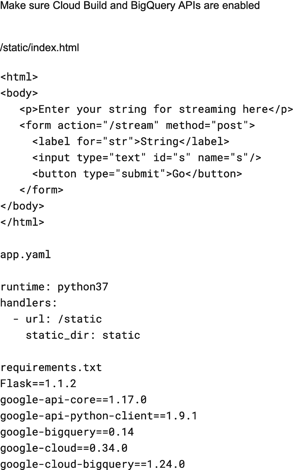
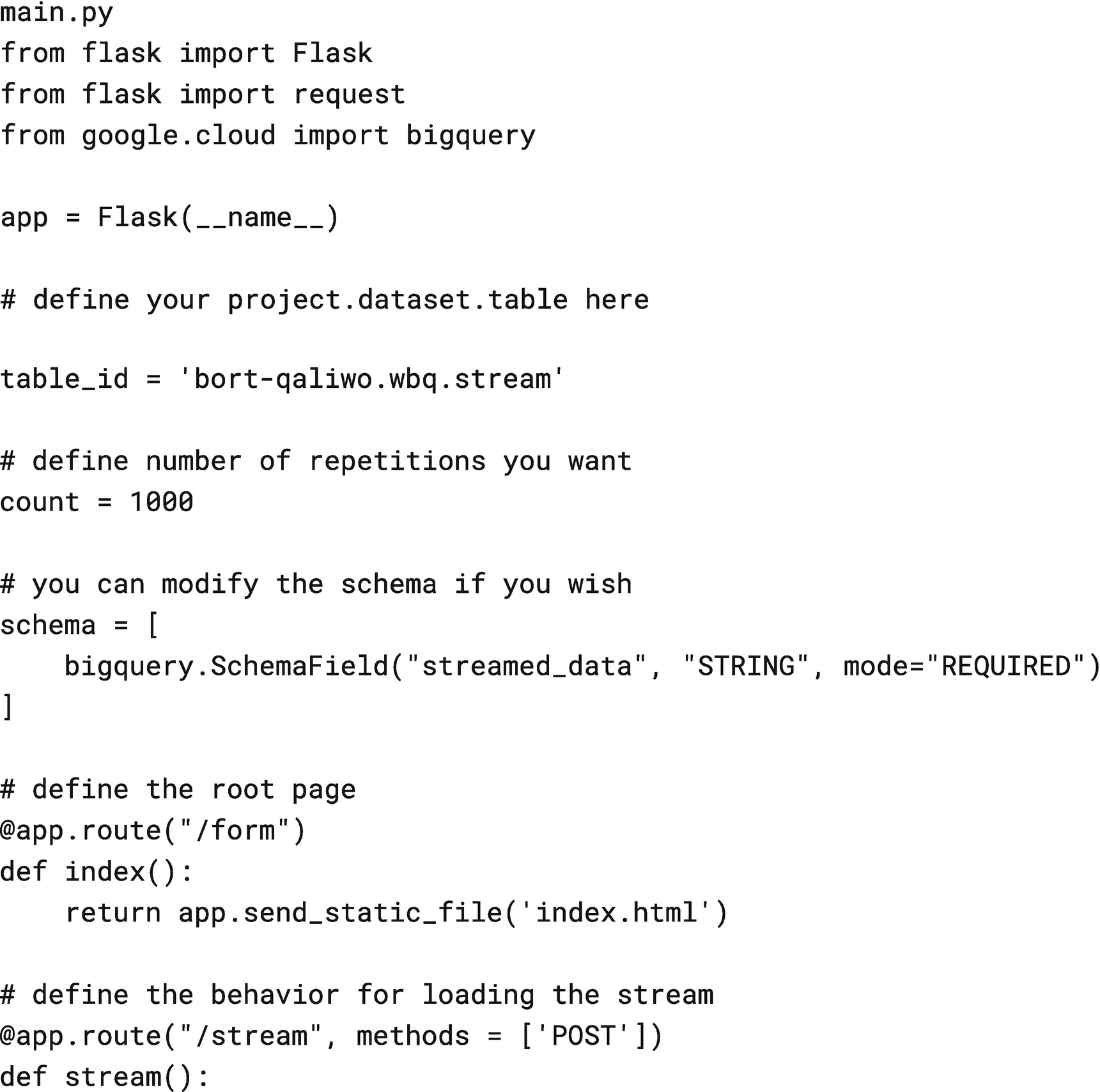
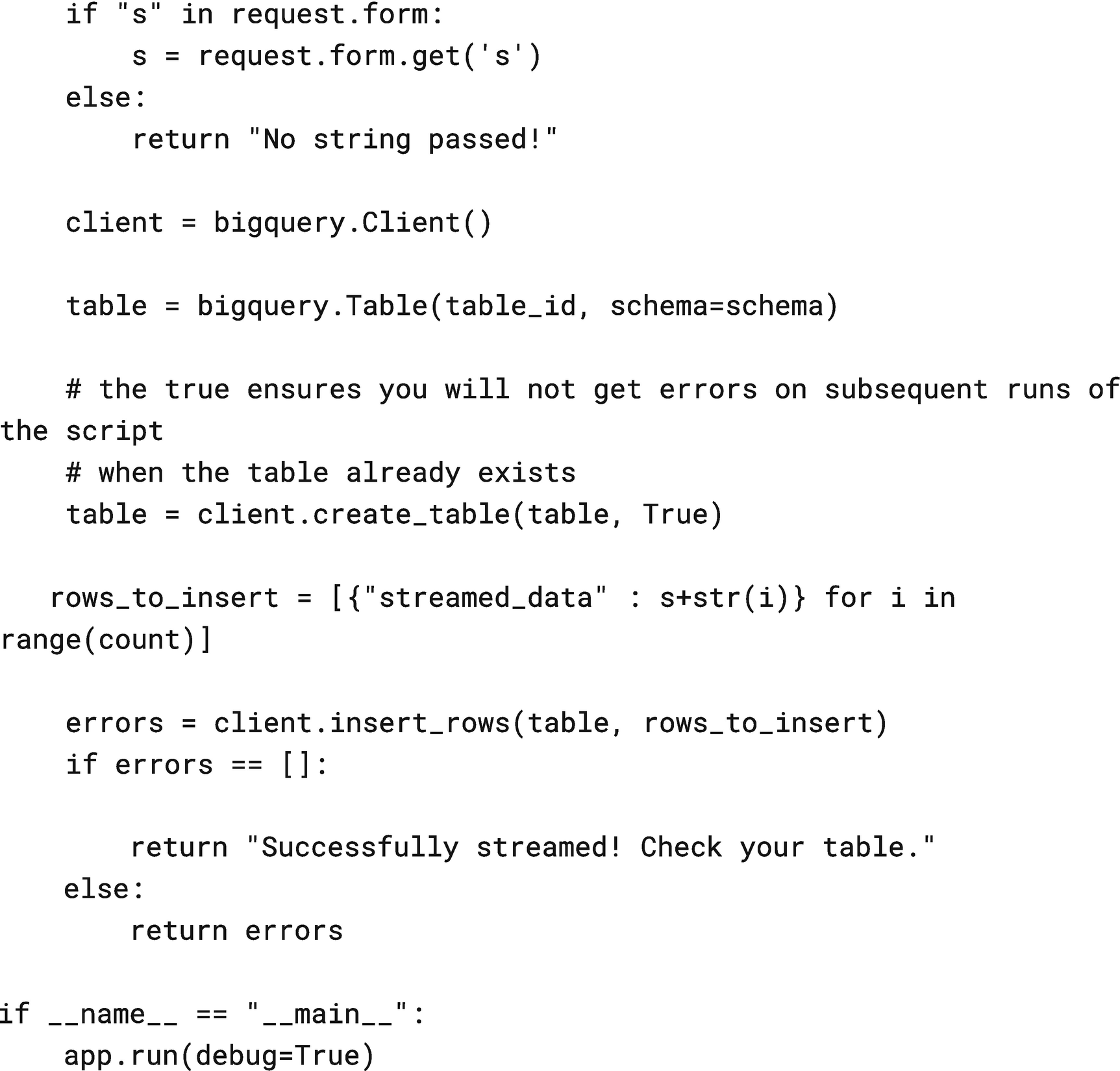
Source code for main.py
Lastly, make sure your requirements.txt has the necessary dependency versions listed for Flask and BigQuery. Yours will be different than mine, so just use whatever the latest is.
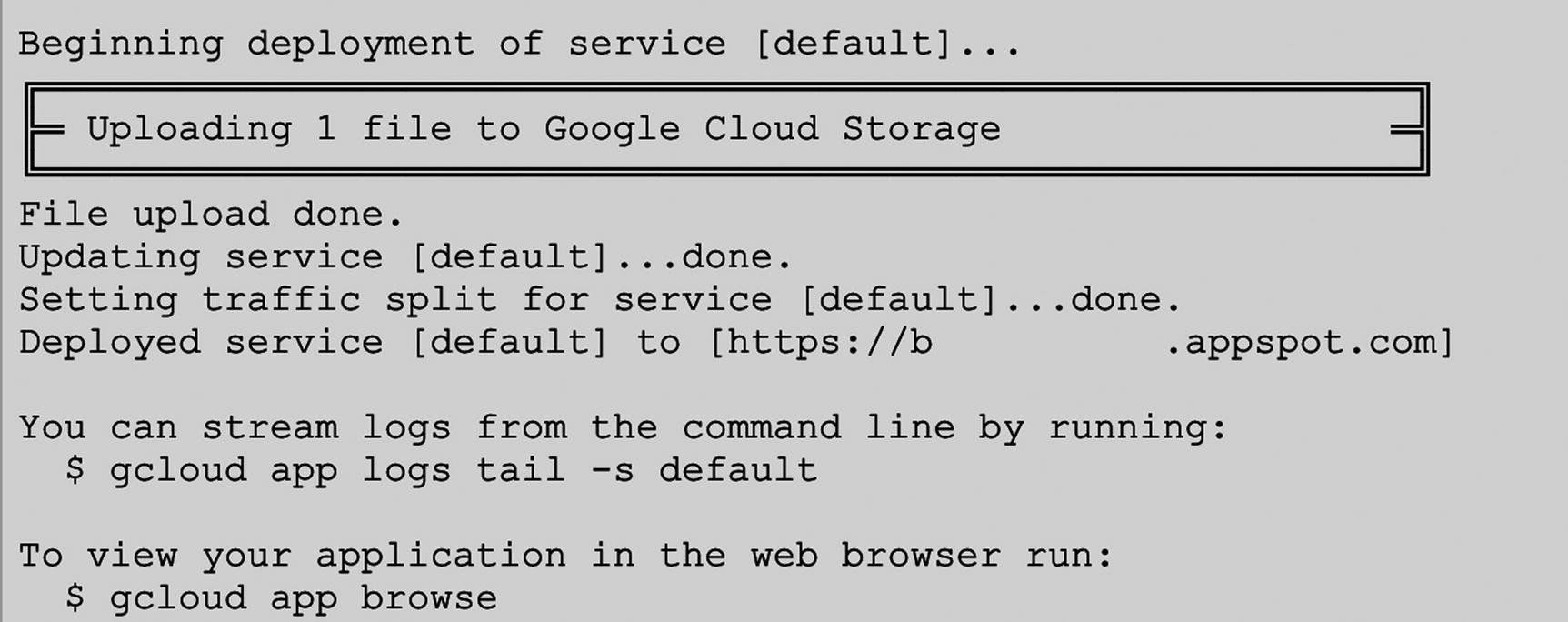
Screenshot of successful deploy
The UI for the sample
Once you do this, the sample will multiply the data and stream it into BigQuery to the dataset and table you specified in your source. Open up a BigQuery console window and select from that table. You’ll see the rows made from the submission you made to the website.
And that’s it! You’ve successfully streamed data!
Common Problems
Of course, it’s not always going to be wine and rows when you’re streaming data to BigQuery. Occasionally, you will run into the messy result of one of the trade-offs you made to support streaming. There are compensation scenarios for all of them, but you have to manage them yourself. Here are a few issues you may run into and some suggestions for compensating for and resolving them.
Insertion Errors
In all cases, when you successfully complete a job, you must inspect the “insertErrors” property to see if any rows failed.
The insertErrors property will typically contain an empty list, indicating everything went fine. If there are rows in there, then you’ll need to programmatically check to see what went wrong in order to repair it.
If some rows indicate a schema mismatch, no rows will have been inserted, and you can jump down to the following “Schema Issues” section. In this case, all the rows you tried to stream will be in the insertErrors list.
If only some rows are in the insertErrors list, you will have to check for the specific failure message to see whether you can simply retry them or if you have to do something to repair them first.
Copying Unavailable Data
If you attempt a copy or export operation before data in your streamed table has become available, the data will be silently dropped from the operation. This could be a major issue if you copy out of a table that has both extant data and incoming stream data without checking.
As mentioned earlier, before you do a copy or export operation, check the _PARTITIONTIME column of all rows in the table to make sure that none of the rows are still in the streaming buffer.
If you are running a scheduled, periodic process on the table, the data will be picked up in a later run. If you have built your process with some tolerance for late-arriving data, this should be sufficient. Combine this with any deduplication strategy to make sure you don’t copy or export the same row twice.
Duplicate Data
In most cases, if you’re using the insertId field, BigQuery will be able to detect any scenarios in which you have to retry the data and automatically deal with the duplication.
In some cases, this may be insufficient. For example, if you used insertId, but waited too long before retrying, BigQuery may have lost track of those particular insertIds and will allow duplication. Google also notes that “in the rare instance of a Google data center losing connectivity,” deduplication may fail altogether. Google just wants to helpfully remind you that BigQuery streaming is not transactional.
So, if you want to be sure your data was not duplicated, you can wait until you have finished the stream and then search for duplicate ID_COLUMNs to clear out the extras. This feels especially inelegant, so I would tend to recommend not even bothering with streaming if you need to go to this end to validate your data. (Dataflow would be a better choice.)
Schema Issues
What happens if you modify the schema of the insert table as you are running a stream? In short, nothing good. If you have changed the schema or deleted the table before you start the job with the old schema, it will fail outright. If you manage to change the schema while the job is in progress, BigQuery should still reject all of the rows and give you information about which rows that conflicted. The rest of the rows, while not inserted, were acceptable and can be retried.
In short, don’t change the schema of tables you are streaming to until you have finished a job and the streaming buffer has cleared. Don’t change a drill bit while the drill is in motion either.
Error Codes
Sometimes the stream will just fail. Most often, this will be due to a network error somewhere between the machine initiating the stream and the BigQuery API. If this occurs, your job will be in an unknown state.
As we discussed earlier, you have two choices here: One, do nothing and accept the uncertainty; or, two, supply the insertId with all of your streaming batches so that BigQuery (or, failing that, you) can attempt deduplication. The first approach is obviously unacceptable for many workloads, so unless you are planning to exceed the 100,000 rows per second quota, use insertId.
If the stream fails right off the bat because it couldn’t connect, you have invalid authentication, or you’re already over quota, the job won’t start and you can safely assume that no rows were inserted at all.
Quotas
If you are running into issues with quotas, the call (or any other call on GCP) will return HTTP code 429: “Too Many Requests.” GCP is generally very good at enforcing quotas right at the published levels, so you can push close to the limit without much risk.
A common pattern for dealing with 429s is to implement an exponential backoff strategy. Often, when implementing such a strategy, you don’t know either the exact rate limit or how many calls you have left to make. In that case, you want to implement a strategy with “jitter,” that is, a random interval tacked onto the backoff interval. Jitter is a good idea whenever a quota is shared by multiple disconnected jobs on the same system. BigQuery streaming quotas are set across your entire project, which means that even if you are only streaming one row per second, if another job is currently monopolizing the quota, your job will still receive 429s. Jitter helps to prevent those disconnected jobs from syncing up with each other and all retrying simultaneously at the same exponential spike.
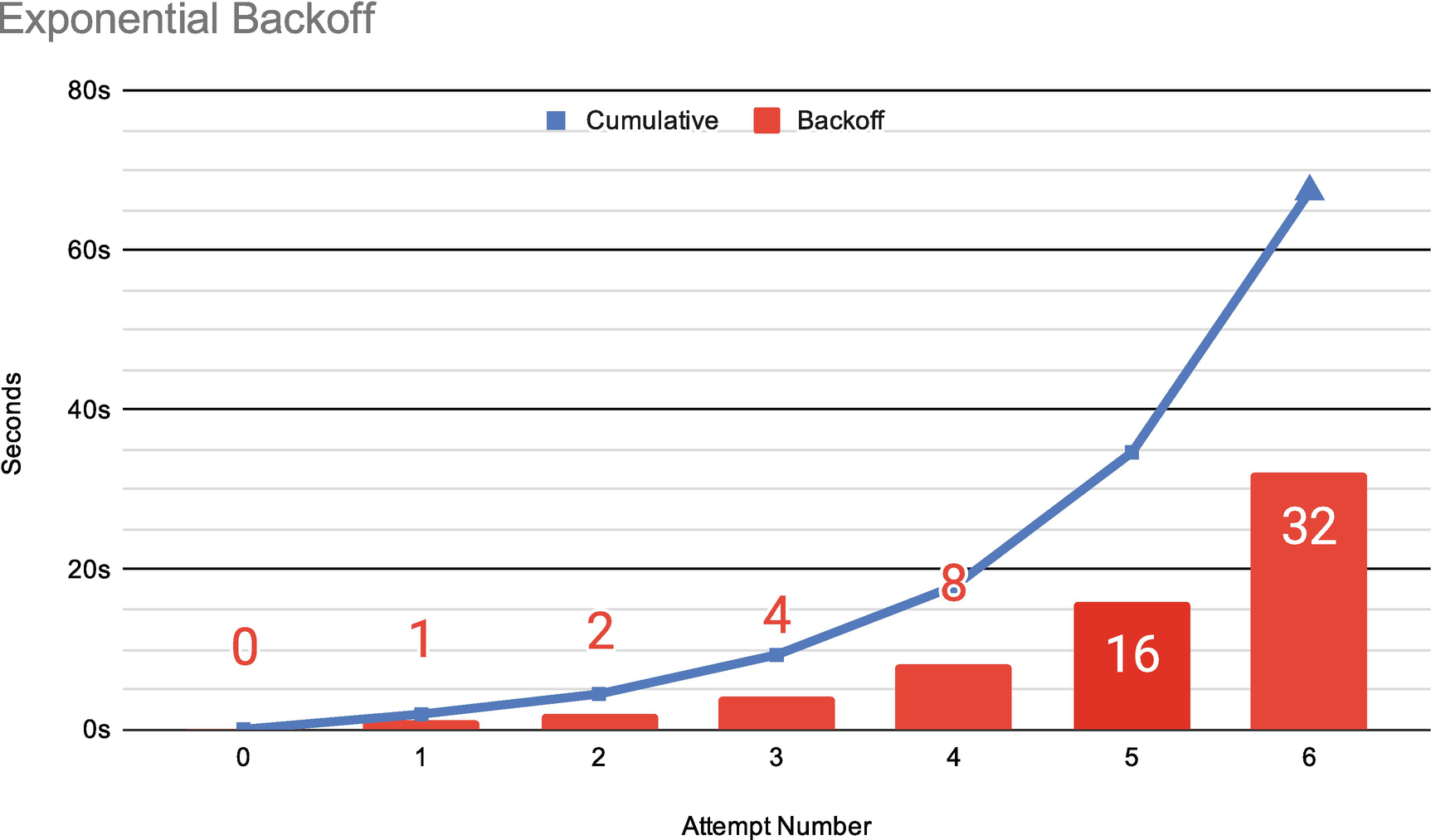
Exponential backoff with jitter calculations
Remember that the intervals should be cumulative, that is, don’t hit it 1, 2, 4 seconds after failure; wait the next interval after each try. Obviously, if the call succeeds, stop retrying.
This strategy will help you balance multiple streaming jobs against each other. What I mean by “syncing” is that if all of your jobs receive 429s simultaneously, without the jitter, they will all retry again at 1 second and likely get the same error.
Lastly, if you are using insertId, cap your exponential backoff rate at 32 or 64 seconds. Since BigQuery is only guaranteed to remember the ID for a minute, going beyond this interval risks additional duplication of your data.
If you’re hitting quotas and you know for a fact that you shouldn’t be, find the other data analyst on your team and tell them to knock it off. If they swear up and down it’s not them, then open a ticket with Google. (I’m serious. While you can look through logs and figure out the source of quota violators, it is usually either you or the person sitting next to you. Save yourself the trouble of doing the forensics and just ask!)
Advanced Streaming Capabilities
There are a few more things you can do with BigQuery streams to prioritize the performance of insertion. You can divide inserts either by date or by a suffix of your choosing. Either will help you maximize accessibility to the data you want to analyze.
Partitioning by Timestamp
Partitioning by date, as covered in Part 1, is also available for streaming applications. This is great if you’re not planning to do additional transformation on the data, but you want it to be available on a partitioned basis for later querying. Since this is done automatically by the streaming job, all you need to do is ensure that you have a DATE or TIMESTAMP column in your insert (and in your destination table), and the streaming buffer will automatically partition the data into the correct tables.
Eighteen-month window: This window (in UTC) starts 12 months before the current datetime and ends 6 months after and is the maximum partitioned range for streaming. If you attempt to partition data outside of this window, the insert will fail.
Ten-day window: This window (in UTC) starts 7 days before the current datetime and ends 3 days after. It is the maximum range for direct partitioning. Data in this range will go directly from the streaming buffer into the correct partition. Data outside this range (but inside the 18-month range) will first go into the unpartitioned table and will then be swept out into the appropriate table as it accumulates.
This emphasizes the use case around temporal data for streaming. While I’ve already broken down the use case around the idea that this should be data that you need available for immediate analysis, this reinforces that that data should be temporally relevant as well.
Here’s a relevant Internet of Things (IoT) example. Let’s say you have a fleet of sensor devices that stream current data to BigQuery. You collect this data on a daily basis into partitioned tables and use it to calculate daily trends. At some point, some of the sensors go offline and stop reporting their data. Several weeks pass as the rest of the sensors continue to report data continuously. Once the sensors are fixed, they begin transmitting the samples that were queued while they were offline. These samples contain new information, but also contain the stale information from the previous couple of weeks. BigQuery will correctly prioritize the relevant, recent information. It will still collect the stale rows, but they’ll accumulate for a while before being partitioned.
Partitioning by Ingestion
The default partition scheme is to insert data into date-based partitions based on current UTC. This assumes either that you have low latency between the event sources and your insertion or that you care more about when the data was received at BigQuery than the event occurrence time.
The preceding sensor example wouldn’t be appropriate for ingestion partitioning, because the event timestamp itself is more important and suddenly reporting stale data as current would presumably cause issues for your metrics collection. However, it’s good for most sampling use cases, like user activity on a live website, logging, or system monitoring.
In fact, when you set up an event sink from something like Cloud Logging (formerly Stackdriver), it also will automatically partition tables by ingestion. For decent performance on large-scale querying of ephemeral data, this is definitely the way to go.
Template Tables
If you want to partition your tables by something other than date, BigQuery streaming supports the concept of template tables to accomplish this. This particular methodology only appears here. BigQuery supported this methodology before it supported date partitioning for streaming, so users would fake out date partitioning using template tables. Now, it is still useful for other partitioning schemes.
To use this methodology, create your destination table to accept stream jobs as you normally would, specifying a schema that will be shared across all implementations of the template. Then, decide what you want to partition by.
In the preceding IoT sensor example, we might choose to partition our inserts by sensor ID instead of date. Or we might want to do two streaming jobs and partition our inserts by date in one table and by sensor ID using template tables. We could also use one or the other method for whatever requires real-time analysis and then copy the data into the other format later on.
Generally, you would want to choose whatever field is the primary key of your data. If you were tracking all movements on an order, you could partition by that order ID. Or you could partition by an account or session ID.
Once you have decided, add your identifier to the call as a templateSuffix. When BigQuery detects that you have supplied both a table name and a suffix, it will consult the table for the schema, but it will automatically create and load into a table in the form tableName+templateSuffix.
To go back to the sensor example, if you used the sensor ID as the suffix, each sensor would supply its insertAll command with its own sensor ID, and BigQuery would take care of the rest, creating tables like SensorData000, SensorData001, and so on.
Summary
Streaming is a technique for inserting data at extremely high velocities into BigQuery with minimal latencies. This speed comes with significant trade-offs, however; data consistency and availability may both be degraded in order to enable inserted rows for analysis as quickly as possible. This method is different from both data loading and Dataflow pipelines and is most appropriate for datasets where you care more about aggregates and trends than about the individual rows themselves. Even when streaming, there are compensatory strategies you can take to minimize the impact of trade-offs. You can also divide inserts by date or a field of your choosing to create a greater number of smaller tables that are easier to query.
We’ve covered two of the methods you can use to get your data loaded into BigQuery. In the next chapter, we’ll cover a technique you can use for loading, migration, streaming, and ongoing data processing, using another Google Cloud Platform service called Dataflow.