Chapter 1 - Back to Basics: What Do You Know Already?
Before you really get going on any journey, it’s a good idea to step back and check what you know already and what tools you already have. This chapter is essentially a refresher chapter. It reminds you about (or reacquaints you with) the basics—the stuff you really need—so you can get your bearings as you head out into the Excel wilderness.
The goal of this chapter is to remind you of what you know already and to fill in any gaps in your basic Excel knowledge. It begins with getting text and numbers into Excel and then moves on to basic functions and some other worksheet basics. If you think you have forgotten any of this material, now is the time to dust it down out of the Excel attic.
This is meant to be a hands-on book, so to play along, open up a blank Excel workbook and get ready to walk through all the step-by-step procedures presented in this chapter.
Note This book shows Excel 2010 in use, but what this chapter covers is true for all versions of Excel (even if you are rocking an Excel 2003 version).
Before you read any further, here are some tips that will make your Excel life a lot easier:
- If you plan to do any calculations with a number, do not put any text in the cell with it. When you mix text with numbers and then try to do calculations, Excel gives you a #VALUE! message.
- Try to keep your entries separate. For example, if you are entering names and addresses, and you think that in the future you may want to sort the names by surname, put first name in one cell and surname in the cell beside it.
- If you need to enter phone numbers or any other numbers that have leading zeros (e.g., 00353111155555), type in an apostrophe (') before entering the number. This is how you tell Excel to treat it as text so that it keeps the first two zeros. If you don’t do this, Excel keeps removing the first two zeros so you get 353111155555. And like a dog playing fetch, you will spend the rest of the day trying to add those two zeros at the beginning.
Note Have I mentioned that I’m Irish? My spelling and some of my examples may be a bit foreign to those of you from the United States and other places. I’m told that U.S. phone numbers never start with two zeros but that a zip code could, in fact, start this way. You may also find other situations where you need to preserve leading zeros.
- Place entries side by side and underneath each other. If you don’t, you create a lot of extra work for yourself. Why? Later on, if all your entries are together and you need to sort or filter your list, Excel will naturally sort and filter all items in the list.
- Before you can format numbers or text, you need to highlight them. The quickest way to do that is to click on the first cell. Then, keeping your left mouse button pressed down, drag the selection down until you have highlighted the cells you want to apply your formatting to.
1. Click in cell B2 and type January. Note that the cursor is flashing at the end of the word.
2. Rest your mouse pointer in the bottom-right corner of the cell, on the fill handle (see Figure 1-1). (I think of it as a soap opera character named Phil Handle.) It should change to a black cross, but if it doesn’t do so, hover the mouse pointer over it until it does.
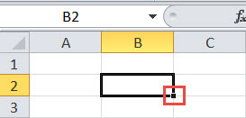
Figure 1-1
3. Holding down the left mouse button, drag the cell down to the cells underneath. You can stop at December, but if you continue, January will reappear.
4. Release the mouse. Holy mackerel! It’s a miracle! Excel has filled in the other months. Yep, that’s how we do it in the Excel world.
Note You can do the same thing with the days of the week: Type Monday in another cell, grab the fill handle, and drag down. Excel fills in the days of the week for you! Sigh, I love Excel.
You can also create your own lists other than the months of the year and days of the week by using the Custom Lists option: Just select File | Options | Advanced | Edit Custom Lists and specify the type of list you want to create.
1. Click in cell D2 and type 1.
2. Click in cell D3 and type 2.
3. Highlight both cell D2 and cell D3 by clicking in the centre of D2. Your mouse pointer changes to a white cross.
4. Drag down the mouse until you see a black line around D2 and D3.
5. Rest your mouse pointer on the bottom-right corner of the cell. (Remember Phil Handle?) It should change to a black cross, but if it doesn’t do so, hover the mouse pointer over it until it does.
6. Holding down the left mouse button, drag down to cell D11. Holy-moly! Excel does the same neat trick with numbers that it does with words. This time, it fills in the numbers 1–10 for you.
Note Practise with other number sequences, such as 10, 20, etc. and 2, 4, etc. Remember that you have to highlight both numbers, or Excel doesn’t know you want a sequence of numbers and just copies the first number, such as 10 or 2, all the way down.
Highlighting More Than One Group of Cells at a Time
1. Highlight the first group of cells you want highlighted (e.g., A2:A4).
2. Press the Ctrl key and keep it pressed down while highlighting the second block of cells (e.g., C2:C4).
3. Release the mouse and the Ctrl key. You now have two ranges highlighted, and when you apply formatting, it applies to both ranges.
Note I refer to tabs frequently in this book. By this I mean the set of icons at the top of the screen. For example, File, Home, and Insert are all tabs on the Excel ribbon.
Formatting Text Entries
1. Highlight the text to which you want to apply formatting.
2. On the Home tab of the ribbon, click on the font formatting you want to apply: B (Bold), I (Italic), U (Underline), etc. (see Figure 1-2). Excel immediately applies the selected formatting to the highlighted text.

Figure 1-2
Note It is worthwhile at this point to have a look at some of the formatting options on the Home tab. Note that when you rest your mouse on each icon, Excel tells you what that icon does. See, Excel is on your side.
1. Enter some numbers into some cells.
2. Highlight those cells.
3. On the Home tab of the ribbon, click on the numeric formatting you want to apply: Currency, Percent Style, Comma Style, etc. (see Figure 1-3).

Figure 1-3
Note There are multiple ways to copy and paste: You can use keyboard shortcuts, right-click with the mouse and use the menu that pops up, or use the Home tab of the ribbon. I show only the ribbon method here, but if you prefer one of the other methods, feel free to continue using it.
1. Highlight the data you want to copy and paste.
2. Click Home | Copy.
3. Click where you want the data pasted.
4. Click Home | Paste (see Figure 1-4).
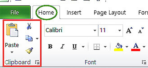
Figure 1-4
|
Survival Tip If you need to copy the same data somewhere else right away, you can just click in the next location and click Paste again. |
Copying Formatting with the Format Painter
1. Highlight the text or numbers that already have the desired formatting.
2. Click Home | Format Painter (see Figure 1-5). A small brush appears on your mouse pointer.
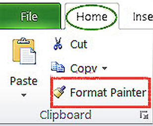
Figure 1-5
3. Highlight the text or numbers you want to apply the formatting to. Excel applies the same formatting to these cells.
Putting the Same Text in Many Cells at the Same Time
1. Click on the first cell you want to add text to.
2. Press the Ctrl key and, keeping it pressed, click on all the cells you want this entry to appear in.
3. Release the Ctrl key. The last cell you clicked is now white.
4. Type the text you want to enter in all the selected cells. (Don’t click again, though, or your selection work will be undone.)
5. When you have finished typing the text for all the selected cells, press Ctrl+Enter. Presto! The text appears in all the selected cells.
Dropping Your Dread of Formulas
When I ask people in class what they want to learn, the answer is invariably “formulas,” which is rather like answering the question “What books do you like?” with “reading.” We’ll get further into the nitty-gritty of formulas later in this book, but in this first chapter, we’ll keep it pretty basic. The following subsections show the basic steps involved in using the basic operators (+, -, /, *, ()) and some essential functions: Sum(), Max(), Min(), Average(), Count(), and CountA(). You will also see how to fix a cell so that it doesn’t move when you copy it and revisit the basics of using worksheets, such as copying, deleting, colouring, etc.
Entering a Formula with the + (Plus) Operator
1. In cell A2, type 100.
2. In cell B2, type 300.
3. In cell C2, which is where you want the answer to appear, type =.
|
Survival Tip Make sure you have clicked where you want the answer to go. I say this because many times I’ve seen people with the right answer in the wrong cell because that is where they had placed the cursor when they began the formula. It’s sort of “right lover, wrong place”. |
4. Click on cell A2 and then type +. Even though you click on the number 100, A2 appears in your formula.
5. Click in cell B2 and press Enter. Even though you click on the number 300, B2 appears in your formula. You now see the answer, 400, in cell C2.
The beauty of doing it this way is that if you decide to change one of your entries, Excel updates the values in the formula for you. For example, if you change the entry in A2 from 100 to 500, Excel changes the answer in C2 to 800.
Copying a Formula Down a Column
1. With the formula you just entered still in place in the workbook, in cell A3, type 50.
2. In cell B3, type 100.
3. Click in C2 and drag the Fill Handle down to copy down the formula. In cell C3, you should now see 150.
Note In this case, you have copied down a formula to only 1 row, but the same process applies if you have to copy it down for 100 rows or indeed 100,000 rows. Enter the formula once and then copy it down.
Entering a Formula with the – (Minus) Operator
1. In cell F2, type 500.
2. In cell G2, type 100.
3. In cell F3, type 1000.
4. In cell G3, type 250.
5. In cell H2, type = and then click on cell F2.
6. Type a minus sign: –.
7. Click in cell G2 and press Enter. You should now see the value 400 in this cell.
8. Copy down this formula, and you should see the value 750 in cell G3.
Entering a Formula with the / (Division) Operator
1. In cell K2, type 1500.
2. In cell L2, type 100.
3. In cell K3, type 1000.
4. In cell L3, type 250.
5. In cell M2, type =.
6. Click on K2, and then type /.
7. Click in cell L2 and press Enter. You should now see the value 15 in cell M2.
8. Copy down this formula, and you should see the value 4 in cell M3.
Entering a Formula with the Multiplication Operator *
1. In cell P2, type 500.
2. In cell Q2, type 10.
3. In cell P3, type 1000.
4. In cell Q3, type 4.
5. In cell R2, type =.
6. Click on cell P2, and then type *.
7. Click in cell Q2 and press Enter. You should now see the value 5000 in cell Q2.
8. Copy down this formula, and you should see the value 4000 in cell R3.
You use brackets in formulas when you need Excel to do a particular calculation before it does other calculations. For example, to calculate the total wages eligible for tax, you need to add basic wages plus overtime first—and you can do that by using brackets.
To see how this works, open the file 01_Brackets. In this file you want to add salary and overtime together and then find 20% of this total. In cell E4, the formula =B4+C4*D4 has been entered and copied down. You don’t have to be an accountant or a tax collector to know that 20% of 8817 plus 215 is not 8860. Of course, if you are a tax collector, you might prefer this number.
Note Throughout this book, I many times ask you to open a particular file to play along with the text. You can find these files at http://www.mrexcel.com/survivalfiles.html. Simply download the files and store them someplace you can easily access.
So what has happened here? Excel has found 20% of 214, which is 43, and added it to 8817…and that’s how you ended up with 8860.
Note Excel does calculations in a very particular way. Before it does anything else, Excel first looks for brackets and does the calculations within those brackets. Then it uses a particular operator precedence: It does multiplication and division before it does addition and subtraction. This is what has happened here. Excel did the multiplication first and then the addition. If you search Excel help for “operator precedence,” you will find a more comprehensive explanation of this concept.
But what you want Excel to do is add salary and overtime together first and then find 20% of that. You do that by using the formula =(B4+C4)*D4 and copying it down. (This formula has already been entered into cell F4 in 01_Brackets.) Now you get an accurate answer: 1806.4.
So remember that if you want to force Excel to do a specific calculation first, put brackets around it.
Getting to Know the Common Excel Functions
A function is essentially a predesigned formula in Excel. There are functions to handle most of the mathematical operations you might want to do. The following sections cover some of the most commonly used functions in Excel: Sum(), Max(), Min(), Average(), Count(), & CountA().
This is not by any means a comprehensive list of Excel functions. However, these are the ones that you will probably use most often. And part of the beauty of these particular functions is that they all operate in a very similar way.
Adding Up with Sum(): This Is Sum-Thing Good
(Sorry, I Do Love a Good Pun)
1. Open a blank Excel workbook.
2. In cell B2, type 500.
3. In cell B3, type 300.
4. In cell B4, type 250.
5. Click in cell B5 and click Home | AutoSum (see Figure 1-6). You now see the formula =Sum(B2:B4) in B5. You should also now see “marching ants” going around the range B2:B4. This means Excel has included all the cells from B2 to B4, inclusive.
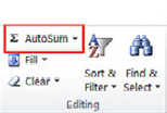
Figure 1-6
Note In Excel, a range is any group of cells, and it’s indicated with a colon between two cells (e.g., B2:B4 for the range of cells from B2 to B4).
6. Press Enter, and you should now see the number 1050. You’ve just used your first function!
All the stuff you have learned already about copying text and numeric data also applies to copying functions.
1. Using the same Excel workbook you just used to try out the Sum() function, in cell C2, type 250.
2. In cell C3, type 300.
3. In cell C4, type 5000.
4. Copy across the Sum() function from cell B5 to cell C5. You should now see the number 5550 in cell C5.
5. Save this file at this point and name it Excel_Practice_1.
Finding the Highest Value with Max()
1. Open the file 01_Functions and in it open the Without Formulas sheet.
2. In cell D6, type =Max. As you start typing, functions appear. After you type M, you get a long list, then after you type MA, the list shortens to the list shown in Figure 1-7.
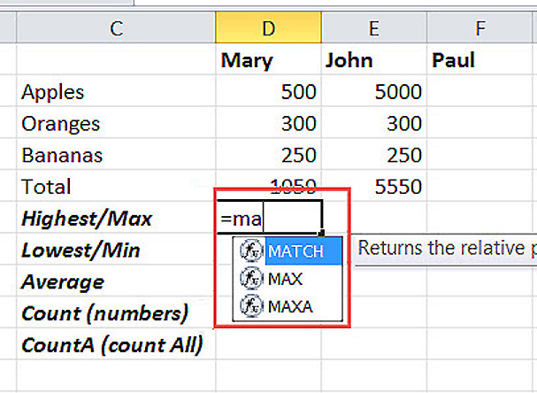
Figure 1-7
3. In the list of functions that appears, double-click Max. =Max( now appears in cell D6.
4. Highlight the range D2:D4 (and note that the marching ants appear).
5. Type ) and press Enter. You now see the highest value in cell D6: 500. At this point, be careful not to include the total figure in cell D6. If you now copy the formula across to E6, you now see 5000 in that cell.
Finding the Lowest Value in a List with Min()
1. Open the file 01_Functions.
2. In cell D7, type =Min.
3. In the list of functions that appears, double-click Min. =Min( now appears in cell D7.
4. Highlight the range D2:D4 (and note that the marching ants appear).
5. Type ) and press Enter. You now see the lowest value in cell D7: 250. If you now copy the formula across to E7, you should see 250 in that cell as well.
Finding the Mean with Average()
1. Open the file 01_Functions.
2. In cell D8, type =Aver.
3. In the list of functions that appears, double-click Average. =Average( now appears in cell D8.
4. Highlight the range D2:D4 (and note that the marching ants appear).
5. Type ) and press Enter. You now see the average value of these numbers in cell D8: 350. If you now copy the formula across to E8, you should see 1850 in that cell.
Finding a Count of Numbers with Count()
1. Open the file 01_Functions.
2. In cell D9, type =Coun.
3. In the list of functions that appears, double-click Count. =Count( now appears in cell D8.
4. Highlight the range D2:D4 (and note that the marching ants appear).
5. Type ) and press Enter. This function tells you how many numbers you have in the list, and you get the answer 3 in cell D9. When you copy it across to E9, you see 3 in that cell as well because there are three numbers in this list.
Counting Something Other Than Numbers with CountA()
Count() is a very pure, unsullied function in the sense that it will only count numbers. But what if you want to count how many names you have in a list, such as Mary, John, and Paul? As you see in the Without Formulas sheet in the 01_Functions file, the Count() function does not give you the desired answer. If you try to use Count() in cell G1 with the range D1:F1, Excel gives you 0 as the answer, not 3, because Mary, John, and Paul are not numbers.
In this scenario, you need to use the CountA() function, which you can think of as the “count all” or “count anything” function.
1. In the same file as in the preceding section, 01_Functions, open the Without Formulas worksheet.
2. In cell G1, type =CountA(.
3. Highlight the range D1:F1.
4. Type ) and press Enter. Excel says the result is 3. Correct!
Amazing People with Excel Number Magic
One of the things I like to do in class is to highlight some numbers on the screen and then proclaim the average and sum of those numbers. I pause a moment to modestly take in the gasps of admiration, pause briefly to bask in the admiration, and then point out that I, you know, read them from the screen. I reassure them that, in fact, I am not Rain Man (from the Tom Cruise and Dustin Hoffman movie about an autistic man who was a mathematical savant). I suppose you would like to amaze friends and strangers like this, too, so I’ll share my secret.
Highlight the numbers on the worksheet and then have a look at the status bar (bottom-left side of screen), where Excel provides answers. The status bar gives you at least the sum and possibly also the average of the numbers you have highlighted (see Figure 1-8). Note that if you right-click on this area as well (in the grey area where the numbers appear), you can see up to six answers: Average, Count, Numerical Count, Minimum, Maximum, and Sum.
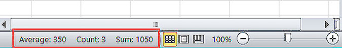
Figure 1-8
If you ever work in an accountant’s office, you need this trick because it’s an invaluable way of checking to make sure your balances are correct.
Understanding the Copying Functions
So far in this chapter, as you have copied a formula, Excel has automatically adjusted it to reflect the layout of the cells you originally gave to the formula. This is what you want most of the time, and it is called relative copying in Excel. The analogy I often give in class is line dancing: When people (or cells) are all lined up to dance and they are told to move to the left, everyone moves to their own left, not to someone else’s left (or at least not intentionally…). So it is with the usual copying in Excel: It follows the pattern of adding up cells as given in the first formula and then replicates that.
However, there are times when you want to use one cell (e.g., a tax rate) with a list of numbers. In that case, you need to make one tweak to your formula to ensure that it doesn’t change as you copy it down. This is called absolute copying in Excel.
The following subsections show these two types of copying in Excel.
1. Open the file 01_Fixing_cells and in it, select the Relative Copying tab.
2. Double-click cell G2. You should see this: =SUM(D2:F2). Essentially, this tells Excel to add up the three cells to the left.
3. Press Enter.
4. Click cell G3. You should see this: =SUM(D3:F3).
The cells listed in the formula in step 4 are different from the ones in the formula in step 2. However, in both cases, Excel is adding up the three cells to the left of the formula. This is relative copying, and it is how Excel usually copies formulas and functions.
Using Absolute Copying to Make Cells Stop Moving
If you want to create a formula that will multiply 10% (in cell H3) by each of the numbers from G4 to G16. If you try your usual copying method first, by clicking cell H4 and entering =G4*H3, you get 10. So far, so good! But now, when you copy it down, it’s not so good. If you check cell H7, you see that it says 240000000. A pay increase of 10% on 400 is not, unfortunately, 240,000,000. (You can insert your currency of choice here.) So what has happened?
As you copied down the formula, Excel moved down the cell references as well. So where you see 240000000, Excel has the formula =G7*H6. You need to do something to stop H3 (10%) from changing as you copy it down. Follow the steps below to see what that something is.
1. In the same file as in the preceding section, 01_Fixing_cells, open the Fixing Cells tab.
2. In cell H4, type the formula =G4 * H3.
3. Press F4. Your formula should now look like this: =G4*$H$3.
|
Survival Tip On some keyboards you must press the Function key (which often has Fn or FN on it) and F4 to activate this combination. |
4. Copy the formula from H4 down to H16. Ah, that’s much better. Cell H16 now reads 130.
Of course, one of the beauties of this technique is that it makes it easier to update your numbers. For example, if you change 10% (in cell H3) to 20%, all your numbers change automatically. Yep, this is another sliver of Excel magic.
Note You can change this F4 configuration to fix a row instead of a cell in a formula (H$3) or fix a column ($H3), but this part of the book is meant to just give you enough to get going. You can see an example of fixing rows and fixing columns in the 01_Fixing_cells file, in the Fixing Rows sheet and the Fixing Columns sheet.
Most workbooks have multiple worksheets in them. Excel refers to worksheets interchangeably as tabs or worksheets or sheets (and I do, too). The following subsections provide quick reminders on how to handle a number of common tasks with worksheets.
To use either of the following methods, open a blank Excel workbook.
On the Sheet Tab
1. Double-click a name of the worksheet you want to rename. It becomes black.
2. Type a new name (e.g., Green) and press Enter. That’s it!
With the Right-Click Menu
1. Right-click anywhere on the sheet you want to rename and select Rename (see Figure 1-9).
2. Type a new name (e.g., Green) into the sheet tab and press Enter.

Figure 1-9
Moving a Sheet Within a Workbook
To try the following methods, you can continue with the workbook you have just been working with.
On the Sheet Tab
1. Hover the mouse over the sheet tab you want to move.
2. Press the left mouse button. You see a tiny black triangle appear to the left of the tab and a page appear at the end of your mouse pointer.
3. Keeping your left mouse button pressed down, drag the sheet to its new location and release the mouse.
With the Right-Click Menu
1. Right-click anywhere on the sheet you want to move and select Move or Copy (see Figure 1-10).
2. In the Move or Copy dialog, under Before Sheet, click the sheet that appears just before where you want to move the current sheet.
3. Click OK.

Figure 1-10
Copying a Sheet Within a Workbook
On the Sheet Tab
1. Hover the mouse over the sheet tab you wish to copy.
2. Simultaneously press and hold the left mouse button and the Ctrl key. A tiny black triangle appears to the left of the tab, and a page appears at the end of your mouse pointer, with + on it.
3. Keeping the left mouse button pressed down, drag the copy to its new location and release the mouse.
With the Right-Click Menu
1. Right-click anywhere on the sheet you want to move and select Move or Copy.
2. In the Move or Copy dialog, under Before Sheet, click the sheet that appears just before where you want to move the current sheet.
3. Select the Create a Copy check box (see Figure 1-11).
4. Click OK.
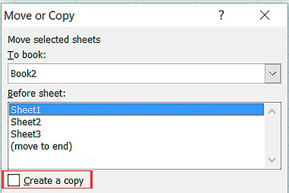
Figure 1-11
1. Right-click the sheet where you want to change the colour and select Tab Color.
2. Choose a colour from the palette (see Figure 1-12). The colour is changed, but you do not really see the change until you click on another worksheet and then return to the one with the changed colour.

Figure 1-12
Note Be careful: This is one move in Excel that you can’t undo.
1. Right-click the sheet you want to delete and select Delete (see Figure 1-13).
2. Click OK. If you have data in the sheet you are about to delete, Excel gives you a warning. Otherwise, it just deletes the sheet.
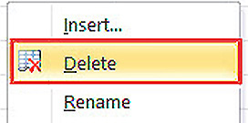
Figure 1-13
Moving a Sheet to Another Workbook
1. Ensure that the workbook to which you want to move a sheet is open.
2. Right-click the sheet you want to move to another workbook and select Move or Copy.
3. From the dropdown list in the Move or Copy dialog, choose the file you want to move the sheet to:
- If you want to move it into a brand-new workbook, choose (new book) from this dropdown.
- If you are moving it into an existing file, under Before Sheet, click the sheet that appears just before where you want to move the current sheet.
Then click OK. Excel moves the sheet, and it no longer exists in the original workbook.
Note This technique is especially useful because if you just cut or copy and paste over data from one worksheet to another workbook, you lose a lot of the formatting (e.g., column widths). But if you move across a sheet this way, the formatting stays put.
Copying a Sheet to Another Workbook
1. Ensure that the workbook to which you want to copy a sheet is open.
2. Right-click the sheet you want to copy to another workbook and select Move or Copy.
3. Select the Create a Copy check box.
4. From the dropdown list in the Move or Copy dialog, choose the file you want to copy the sheet to:
- If you want to copy it into a brand-new workbook, choose (new book) from this dropdown.
- If you are copying it into an existing file, make sure you have selected the destination file in the dropdown list at the top and then, under Before Sheet, click the sheet that appears just before where you want to move the current sheet (see Figure 1-14).
5. Then click OK.

Figure 1-14
Please put down the scissors, staples, glue, and sticky tape and step away (slowly) from the photocopier. Something that comes up over and over again in classes I teach is the perennial problem of printing. Oh yes, I mention scissors, glue, and staples, and inevitably a few heads start to bob and wry smiles appear. Often when you print in Excel, what you want to print does not fit on the page—and the glue and scissors invariably get whipped out. (The cynic in me wonders if, in fact, the glue is needed after the stress of the entire process….) There’s got to be a way around this, right? Right.
Well, the main thing you need to remember is that most of what you need for printing is available on the Page Layout tab (see Figure 1-15).
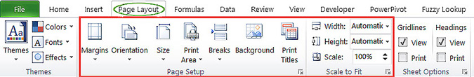
Figure 1-15
Fitting a Worksheet on a Printed Page
1. Open the file 01_Printing_sample.
2. View the file in Print Preview (either by selecting the view from the Quick Access toolbar) or by selecting File | Print. You can now see how the printed file will look, without actually having to send it to the printer. Notice that the file wants to print on 26 pages, and you are missing the heading ScdStartDate (see Figure 1-16).

Figure 1-16
In fact, if you keep going through the pages, you will find that ScdStartDate has decided to declare itself an independent republic and print itself on pages 15 onward. (You reached for your scissors, glue, and sticky tape, didn’t you? Please put down all those implements quietly as you learn how to do this in a much easier way.)
3. To make everything fit on the printed page in this case, select the Page Layout tab and find the Width dropdown in the Scale to Fit options section (see Figure 1-17). In it select 1 page instead of Automatic.
4. Check the file in Print Preview. The document is now going to print on 11 pages, and ScdStartDate has rejoined its comrades, where it belongs. Magic!
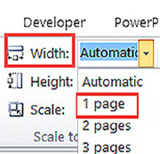
Figure 1-17
Note If you have a document that will not fit tidily onto the desired number of pages, fix it with the Width option on the Page Layout tab.
|
Survival Tip To make a smaller spreadsheet appear bigger than it is, increase the % size in the Scale box on the Page Layout tab (see Figure 1-18). |
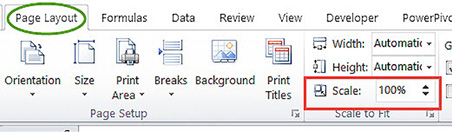
Figure 1-18
Printing Headings on Every Page: A Title! My Spreadsheet for a Title!
1. Keeping the file 01_Printing_sample open, view the file in Print Preview. Notice that headings appear on the first page but don’t appear on the following pages. This is a nuisance.
2. Select Page Layout | Print Titles (see Figure 1-19).
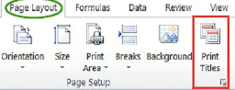
Figure 1-19
3. In the Page Setup dialog that appears, click in the Rows to Repeat at Top box (see Figure 1-20).

Figure 1-20
4. On the actual spreadsheet, click on the row number (on the left side of the screen) that has the headings you want to repeat at the top of every page; in this case, click row 1. You now see $1:$1 in the Rows to Repeat at Top box in the dialog.
5. Check the file in Print Preview again. The headings now appear at the top of every page.
|
Survival Tip If you have a spreadsheet with multiple columns, and you want the first column to repeat on every page, choose Page Layout | Print Titles. Then select the Columns to Repeat at Left box and highlight the columns you want to appear on the left side of every page. |
1. Highlight what you want to print and select Page Layout | Print Area | Set Print Area (see Figure 1-21).
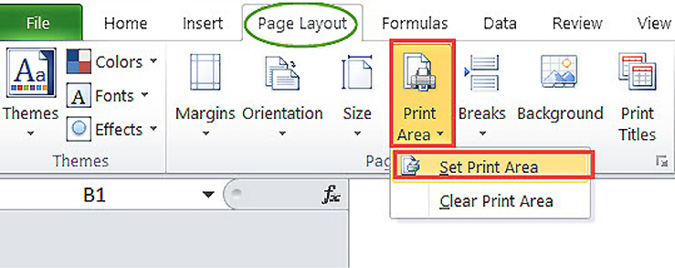
Figure 1-21
2. Print as you normally would.
3. When you are finished printing, select Page Layout | Print Area | Clear Print Area (see Figure 1-22). Next time you choose to print this worksheet, you will print the whole thing, not just the selected print area.
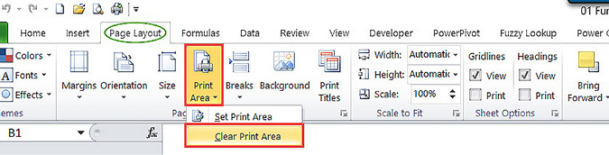
Figure 1-22
Note If you do not clear the print area, Excel prints out just this specific selection the next time you print the worksheet.
1. To change the page orientation from Portrait to Landscape, select Page Layout | Orientation | Landscape.
2. To change the page orientation from Landscape to Portrait, select Page Layout | Orientation | Portrait (see Figure 1-23).

Figure 1-23
Breaking up is not hard to do—for pages. Use the following steps when you need page breaks at points in a spreadsheet that Excel does not consider “natural” page breaks.
1. Click where you want a page break to go.
2. Select Page Layout | Breaks | Insert Page Break (see Figure 1-24). Yep, it’s that simple.
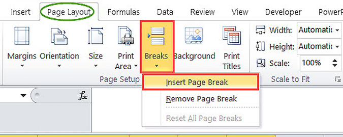
Figure 1-24
1. If you find that a page break doesn’t work for you, click on the spreadsheet beside the break (or underneath, if it’s a horizontal page break) and then select Page Layout | Breaks | Remove Page Break.
2. If you have inserted many page breaks and you now have no idea what is working or not, select Page Layout | Breaks | Reset All Page Breaks to restore the spreadsheet to its original, natural, page breaks.
What if you want your name, the filename, a page number, or where you put the file to appear on every page? What if you want to make it clear that you own this spreadsheet? In this case, you add a header or footer—or both.
1. Select Page Layout | Print Titles (see Figure 1-25).

Figure 1-25
2. In the Page Setup dialog box that appears, select the Header/Footer tab (see Figure 1-26).

Figure 1-26
3. To make your name appear at the top of every page, choose an option from the dropdown list. You can choose from a number of choices, including filename and path, your name, and date (see Figure 1-27).
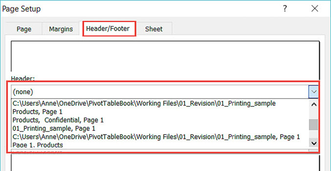
Figure 1-27
4. If you want the date to appear at the bottom of every page, choose Date from the Footer dropdown.
Adding a Picture in the Background
At some point you might want to add a favourite picture or motivational quote as a background to a spreadsheet. When you do this, the background picture doesn’t actually print with your worksheet, but it does appear onscreen.
1. Select Page Layout | Background (see Figure 1-28).
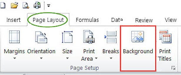
Figure 1-28
2. Browse to a folder where you have photos stored and select a photo.
3. Click OK. Your selected photo now appears as the background for the entire worksheet—all million-plus rows of it.
4. To remove the picture you added, select Page Layout | Delete Background (see Figure 1-29).
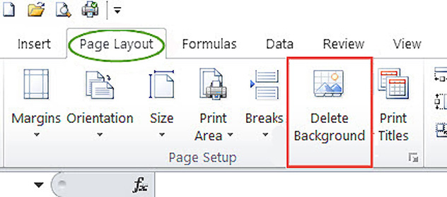
Figure 1-29
Rob Collie once observed in a blog post that Excel lovers tend to fall into two camps. One camp declares “I want a chart with that!” to everything. The other camp (the one I fall into, I confess) has a secret hankering for formulas and doesn’t love charts so much. However, since most of the business world falls into the first camp, you need to be able to add at least basic charts to your spreadsheets.
The following sections cover creating basic column charts, pie charts, and combination charts.
|
Survival Tip When you’re making a chart, use the Ctrl key to select only the data you need. By this I mean highlight the first range. Then press the Ctrl key and, while keeping Ctrl pressed down, highlight the other ranges you want to include. Oddly enough, charts often work better if the top-left cell is blank; this is particularly the case with column and bar charts. |
I want to emphasise that this chapter provides just an introduction to charts. Also, the approach I suggest here is really only suitable for smaller data sets. If you have much larger data sets, I suggest that you make a pivot table and then extract a pivot chart from it. (You’ll learn about this in Chapter 5, “Creating Pivot Tables.”)
1. Open the file 01_Chart_demo.
|
Survival Tip Think about exactly what you want your chart to show. (In this case, you want to make a column chart that shows the amount of money spent each day). Then make sure you highlight only the data you need. (In this case, you need just the Date and Amount columns.) Keep in mind that in some situations, you may need to use your Ctrl key to select only the data you need. |
2. Click the Date heading and press Ctrl+Shift+Down Arrow to highlight the entire Date column.
3. With the Ctrl key pressed, click the Amount heading. While still holding down the Ctrl key, also press Shift+Down Arrow to select the Amount column in addition to the Date column.
4. Click Insert | Column and choose the first chart in the list—the clustered chart in the 2-D Column section (see Figure 1-30).

Figure 1-30
5. Release the mouse. That’s it: Excel creates your column chart. Excel also gives you some new ribbon tabs at the top right of the screen: Design, Layout, and Format (see Figure 1-31).
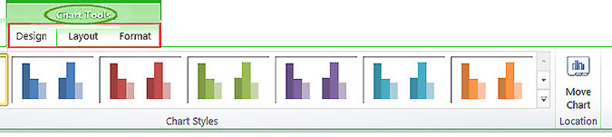
Figure 1-31
|
Survival Tips Click on the Design tab and note that you have a veritable gallery of different chart types in the Chart Styles section. (At this point, be sure to pause to consider that you are now poised to join the pantheon of Excel gods and goddesses you have admired with their gee-whiz charts.) It is worthwhile to experiment a bit with them. You also have options to the left on the Design tab for changing the chart layout. Here’s another trick to help you with chart creation: When you have finished creating a chart, you can click on it and then click Design | Switch Row/Column to change around the layout of the data (see Figure 1-32). |

Figure 1-32
6. Practise creating another column chart, this time with the Payee and Amount columns.
It’s really important to understand that a pie chart is suitable for showing just one set of numbers, ideally where the headings are unique (e.g., gender breakdown of employees in a company).
1. To construct a pie chart for category and amount, open the sheet called Pie Chart in the file 01_Chart_demo.
2. Highlight the headings in A1 and B1 and press Ctrl+Shift+Down Arrow to highlight all the headings and amounts.
3. Choose Insert | Pie | 2-D Pie | Pie (see Figure 1-33). Now you have a pie chart.

Figure 1-33
4. To add percentages to the pie chart, click on the chart and select Design | Chart Layouts (to the left of the Chart Styles) and select a layout, such as Chart Layout 1, which adds percentages and labels to your pie chart.
A combination chart includes two or more types of charts. A common type of combination chart is a column chart with a line in it to show something like targets. This chart type is beloved by many organisations, so it’s useful to know how to make it.
Now, I’m going to be a bit unorthodox here in that there are better ways to create charts than the one I’m about to show you. But this book is not called How to Be a Wonderful Chart Creator. It’s called Excel Survival Guide, and it’s about ways to quickly get through typical Excel scenarios.
1. Open the Combination worksheet in the 01_Chart_demo file.
2. Assuming that you have set a daily total of 500, and you want that to appear as a line on your chart, add an extra column called Target that has 500 repeated all the way down (see Figure 1-34).
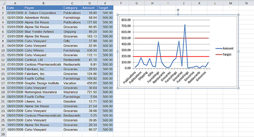
Figure 1-34
3. Highlight the three column headings Category, Amount, and Target and select Insert | Column | 2-D Column | Stacked Column (yep, living dangerously!).
4. To convert the Target part of the chart into a line chart, click one of the red columns. Note that small circles (I often call them Mickey Mouse ears) appear on all the red headings (see Figure 1-35). (If you’re reading the print version of this book, I’m sorry to say you can’t actually see the red colour. But trust me: It’s there. And you can see the small circles in Figure 1-35.)

Figure 1-35
5. Select Design | Change Chart Type (see Figure 1-36).
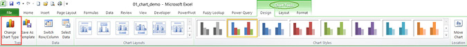
Figure 1-36
6. Select Line | Line. You now have a horizontal line for your target.
Note Jon Peltier (http://peltiertech.com) provides a much more comprehensive tutorial on creating a chart like this. In his version, the horizontal line actually stretches all the way across. However, as a first quick step, what I show here will get you started.
I’m about to let you in on a dirty little secret about lines on charts. More than once people have admitted to me that they just drew the line. I know you want to know how to do this small cheat, so I’m going to tell you how:
1. It’s easiest if you have gridlines on your chart, so make sure you have them by clicking on the chart and selecting Layout | Gridlines | Primary Horizontal Gridlines and clicking Major Gridlines.
2. Identify the point on the chart where you want the line to go. It’s probably best to align the horizontal line with one of the gridlines.
3. Select Insert | Shapes and select a line type.
4. Click and drag the line across the chart. Hey, you have your line!
5. To change the colour of the line, click the line and select Format | Shape Outline and select a colour.
6. To change the weight of the line, select Format | Shape Outline | Weight and click the line with the desired thickness (e.g., 3pts).
Of course, before you complete this chapter, I need to mention keyboard shortcuts. An important part of using Excel effectively is having a repertoire of Excel shortcuts for navigating around. Here’s how I recommend you build such a repertoire:
1. Choose one or two shortcuts a week, starting with shortcuts for stuff you do frequently, such as cutting and pasting (Ctrl+X and Ctrl+V) and inserting and removing columns (Ctrl++ and Ctrl+-)
2. Work on these new-to-you shortcuts all week, until by the end of the week they are in your muscle memory.
3. The following week, repeat steps 1 and 2 with a new set of shortcuts.
By the end of a couple of months, your speed and efficiency in navigating around Excel will have improved considerably.
Table 1-1 lists the most common Excel shortcuts. I’ve chosen these shortcuts because you will probably be working with large (thousands-plus) data sets, and if you do not use them, you will spend chunks of your life scrolling painstakingly down to the end of your sheet and then equally laboriously crawling to the top again—like someone coming up slowly from the bottom of the ocean.
Table 1-1: Excel Shortcuts
|
Shortcut |
Description |
|
Ctrl+Down Arrow |
Moves to the bottom of the list (assuming no spaces) |
|
Ctrl+Up Arrow |
Moves to the top of the list (assuming no spaces) |
|
Ctrl+Right Arrow |
Moves to the extreme right of the list (assuming no spaces) |
|
Ctrl+Left Arrow |
Moves to the extreme left of the list (assuming no spaces) |
|
Ctrl+Shift+* |
Selects the entire list (Thanks to Chandoo at http://chandoo.org for this one!) |
|
Ctrl+Home |
Moves to A1 from anywhere in the spreadsheet |
|
Ctrl+End |
Moves to last cell clicked in the spreadsheet (like moving to the furthest footprint on newly fallen snow) |
Of course you can find many more keyboard shortcuts at the Microsoft site.
This chapter covers the basics of Excel: data entry, formulas, fixing cells, printing, charts, and worksheet housekeeping. If you can do this much with speed and grace, you are already ahead of many Excel users. Knowing this stuff will make you a hardy Excel survivor. If you continue through the following chapters, you will become an Excel thriver.