Chapter 4 The Vlookup() Function: An Excel Essential
Here’s a question I often get asked in class: “I’ve got matching data in two locations that I have to use together. Why can’t I just copy and paste any new data when it changes?”
Does your data change? I suspect the answer is “er, yes.” In that case, you could copy and paste, but it’s much smarter to use the Vlookup() function to capture the changes.
If you use Copy and Paste to insert data instead of using Vlookup(), you will have to manually update your spreadsheet. That means locating the place where the data changed, copying the data, and then pasting it in to your own spreadsheet.
This isn’t a robust method of updating a spreadsheet. For example, what happens if you forget what data you have copied and pasted into your spreadsheet? And what happens if the new data isn’t in the same order as it was before? Yep, speaking from experience here, that’s when you will have officially made a dog’s dinner of your data, and that is not a good thing.
It’s worth learning how to use Vlookup() because with this function, your data is automatically updated, so it’s always accurate and safe.
Essentially, the Vlookup() function allows you to match up the same data from two different data sources. It is used for many Excel scenarios, and knowing how to use it properly will save you time and grief.
Your data sources could be on the same worksheet, in separate worksheets in the same workbook, or—as is often the case—in different workbooks. We will look at each of these situations in this chapter.
In terms of your Excel survival, the Vlookup() function is like your water bottle. It’s a lifesaver. However, it does have a few idiosyncrasies you need to be aware of.
Understanding the Vlookup() Function Syntax
Here’s the syntax of the Vlookup() function (which you can find yourself by selecting Formulas | Lookup & Reference | VLOOKUP; see Figure 4-1):
Vlookup(Lookup_value,Table_array,
Col_index_num,Range_lookup)

Figure 4-1
Okay, don’t panic. Let’s just walk through it.
I want you to imagine a scenario that will make it easier to understand the structure above: You are buying a bottle of water in your favourite supermarket. It will be scanned through the till system using the barcode. Next, the till will check this barcode against the supermarket’s master list of products so it can update the stock list and charge you the correct amount for the water. This all happens so that your receipt will show the correct description and price for your bottle of water.
Here’s what happens: The till checks the barcode on the bottle (that’s the Lookup_value) and compares it to the master list of products. For this to work, the barcode has to be in two places (i.e., on the bottle and in the supermarket’s master list of products).
The till system goes to the supermarket master list of products (Table_array) and gets the number of the column in that list that holds the description (Col_index_num) of the product. It then goes through the same process again to get the price. This is how the correct description and price for your water get onto your receipt.
The till system is then told that if it wants an exact match between the barcode on the bottle and the barcode in the supermarket database, it needs to refer to Range_lookup.
Note Setting Range_lookup to FALSE ensures that the two data sources get an exact match. You can also leave Range_lookup blank in scenarios where you don’t want an exact match. A good example of this is when you want to match an exam mark to an exam grade. Let’s say Joe Bloggs gets an exam mark of 92%. His grade is assigned based on the fact that his mark falls into the 90%–100% range. When this happens, Joe is assigned an A for the exam. To set up a Vlookup() function for this, you would make sure that anyone who gets an exam mark between 90% and 100% gets an A. Unlike in the barcode example, here you do not want an exact match between 92% and the A grade result because this would mean that only anyone who gets exactly 92% would get an A grade. Also, it would assume that Table_array will always be listed alphabetically. To see how this is done, check out the file 04_Vlookup()_true.
Troubleshooting Vlookup(): Dealing with #N/A Errors
Before getting into the sections that present situations where you use Vlookup(), this section provides some tips on avoiding frustration while using Vlookup(). Of course, functions don’t always work smoothly, and here we look at some of the troubles you are most likely to meet.
Anyone who has ever done a Vlookup() has experienced #N/A errors. What can you do to keep the number of these problems to a minimum? I usually suggest thinking of these three Ls:
- To the left
- Like
- On the same line
Here’s what I mean by this: The Lookup_value has to be to the left of your formula, identical to (like) the first column of the table, and on the same row (or line). And here are even more details:
- To the left means the lookup value needs to be to the left of your formula (or, if you imagine a clock, think of the 6:00 to 12:00 portion of the face), on the same line. Note in the Situation 1 example later in this chapter that the SalesTerritoryKey is to the left of the Vlookup() formula that begins in cell I2.
- Like means the lookup value should be identical to the first column of the Table_array. Note that the matching column (i.e., the value in Lookup_value) has to be the first column of the table (or, as I like to joke in class, it doesn’t have to be, but it doesn’t work otherwise!).
This means your data types must be the same. For example, if your lookup value is a number, and Excel is reading it as text, prepare to see many many #N/As because the Vlookup() function thinks they have nothing in common and refuses to work. You can check that your number is not text by clicking on the cell you want to check. Next, select the Home tab and ensure that the Number group says General or Number and not Text. If it says Text, and the matching value in your Table_array is a number, the Vlookup() will not work. If data is text, this is indicated by the green marker in the top-left corner of the cell. If you click it, you get the option Convert to Number or Convert to Text, which you can use to convert your data so that the data types of both the Lookup_value and the first column of the Table_array are the same.
In addition, the entries in the first column of the table array have to be unique. This may sometimes require the creation of a helper cell (which is covered later in this chapter).
- On the same line really means “on the same row,” but to make this little memory aid, I wanted a third L here.
If any of these conditions are not met—particularly either of the first two—you will probably have trouble with your Vlookup().
Understanding When to Use Vlookup()
The following sections describe a few situations when you should use Vlookup():
- Situation 1: Matching up data in the same worksheet and file
- Situation 2: Matching up data in the same file but different worksheets
- Situation 3: Matching up data with a formula and table array in two different files
Obviously, these are not the only ones, but they are very typical ones.
Situation 1: Matching Up Data in the Same Worksheet and File
In this section, you’ll see how to use Vlookup() to match up data in the same worksheet. The files you need for this section are in the Working Files folder. In this example, you will pull in SalesTerritoryCountry starting at cell I2 for the SalesTerritoryKey. Your matching list will be coming from A1:E12 on the same worksheet.
1. Open the file 04_Vlookup_same_worksheet.
2. Click the Sales Territories sheet.
3. Click in I2 and select Formulas | Lookup | Reference | VLOOKUP.
4. In the Function Arguments dialog that appears (see Figure 4-2), click in the Lookup_value box and click in H2.
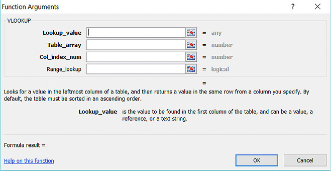
Figure 4-2
5. Click in the Table_array box, highlight the part of the spreadsheet that contains the data (A1:E12), and fix the range by pressing F4 to apply dollar signs to it. You now see $A$1:$E$12 in the Table_array box.
Note It is very important that you fix the range by pressing F4. If you don’t, the range will change as you copy down the formula, so it will start reading A2:E13 as you copy it down.
6. Click in the Col_index_num box and type 4 (because SalesTerritoryCountry—the data you want to pull in—is the fourth column from the left in the Table_array part of the formula).
7. In the Range_lookup box, type False. This means you want an exact match, regardless of how the first column of the Table_array bit is sorted. Excel tends to assume that the first column of the Table_array list will be sorted alphabetically, but that is not always what you want.
8. Click OK, and you should see United States in cell I2.
9. Press Enter to copy down the whole formula.
10. Test the formula by changing D10 (sales territory 9) from Australia to Ireland. You now see this change reflected in cell I10. In cell I10, you now see Ireland. Change it back to Australia. As you can see, any changes in the Table_array portion are reflected in the answers to the formula. So the changes happen automatically.
Situation 2: Matching Up Data in the Same File but Different Worksheets
Sometimes you need to match up data when a formula is stored in one worksheet and a table array is stored in a different worksheet. The approach in this situation is nearly identical to the approach you take when you’re matching up data in the same worksheet and the same file. In this case, you mainly just need to remember that your formula and table array are in the same file but on two different worksheets. However, I recommend taking an additional step to make your life a lot easier in this case: Take advantage of the ability to view multiple worksheets on the same screen.
1. Open the file 04_Vlookup_separate_worksheets.
2. Select View | New Window (see Figure 4-3) to create a window for each additional worksheet you want to see. (For example, if you want to see your current worksheet and two others, select View | New Window twice.) A number corresponding to the number of windows appears after the filename (e.g., you see 04_Vlookup_separate_worksheets: 3 if you have three windows).

Figure 4-3
4. In the Arrange dialog that appears, check Windows of Active Workbook to view all the worksheets on the same screen and leave Tiled selected (see Figure 4-4). You can now view two files side by side.

Figure 4-4
Closing Extra Windows
If you find that you have been a little too enthusiastic in clicking New Window, and it looks as though windows have started to reproduce, you need to close some windows.
1. Click in the window you want to close and then click the X at the top-right of the window to close it.
2. Repeat until you have open only the windows that you require.
3. Select View | Arrange All.
4. In the Arrange dialog that appears, leave Tiled selected.
5. Click the sheets you want to view— Sales Territories and Enter Formula on This Sheet—so you can see them at the same time. Sales Territories should be visible on one side, and Enter Formula on This Sheet should be visible on the other, as shown in Figure 4-5.
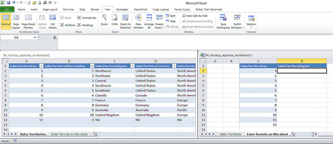
Figure 4-5
6. In the sheet called Enter Formula on This Sheet, click in D2 and select Formulas | Lookup & Reference | VLOOKUP.
7. Click in cell C2 in the same worksheet.
8. Click in the Table_array box in the Function Arguments dialog, highlight the worksheet (Sales Territories) that contains the data from A1:E12, and fix the range by pressing F4 to apply dollar signs to it.
Note It is very important that you fix the range by pressing F4. If you don’t, the range will change as you copy down the formula, so it will start reading A2:E13 as you copy it down.
9. Click in the Col_index_num box and type 3 (because SalesTerritoryRegion—the data you want to pull in—is the third column from the left in the table_array part of the formula).
10. In the Range_lookup box, type FALSE.
11. Click OK and copy down the formula to D12. You should now see Northwest in D2 and other regions entered in the range D3:D12. (The last entry should be United Kingdom in D12.)
Situation 3: Matching Up Data in Two Different Files
Before you start looking closely at this situation, here are some things to consider:
- Having all the files that relate to a Vlookup() in one folder generally reduces the number of problems with broken links. You can check what files you are using by selecting Data | Edit Links. In the Edit Links dialog that appears, make sure you are in the file that is pulling in the data from the other files (see Figure 4-6).

Figure 4-6
- Make sure both files involved in the data matching are open. If they are not and you already have a Vlookup() function created, you may see the REF! message when you open the file that contains the Vlookup() function.
- Make sure you are in the file that is pulling in the data from the other files.
- Sometimes if you get the REF! message, it just means the file needs to be opened. Use an Iferror() function around it to say “please check that the file is open.” (You can read more about this function in Chapter 3, “Further Cleaning, Slicing, and Dicing.”)
- When you are selecting your table array and it is in another file, dollar signs appear automatically on the range you have selected. Of course, a better idea is to convert your table array to a table, as discussed later in this chapter.
Get ready to rumble—or at least get your files visible—and follow these steps:
1. Open the two files 04_Sales_territories and 04_Vlookup_functions_files. Ensure that all other spreadsheets are closed.
2. Select View | Arrange All, and in the Arrange dialog that appears, ensure that Windows of Active Workbook is not selected and leave Tiled selected. Your two files should now be open and placed side by side.
3. Click in cell B2 in the 04_Vlookup_functions_files file.
4. Follow the steps in the section “Situation 2: Matching Up Data in the Same File but Different Worksheets” to have your Vlookup() pull in SalesTerritoryRegion. However, this time, when it comes to the table array, highlight the column heads SalesTerritoryKey, SalesTerritoryRegion, SalesTerritoryCountry, and SalesTerritoryGroup in the 04_Sales_territories file and then press Ctrl+Shift+Down Arrow. The filename now comes into the formula. In this version, it is =Vlookup()(A2,'sales territories.xlsx'!Sales[#All],3,FALSE), but in your file, it will probably be different because you will have it stored in a different location.
5. Copy down the formula to B13. You can check your answers in the sheet called Completed.
How to Solve Common Vlookup() Problems
Alas, while the Vlookup() function is immensely useful, it doesn’t always work as expected, and in this section I cover some of the most common issues.
The most common reason that you end up with missing data is that your table array has not been extended to include the new data (e.g., a new sales territory) that you have added to the list with the lookup value.
1. Open the file 04_Vlookup_missing_data. If you look in cell I11, you see #N/A.
2. Click on the formula, and you see that the table array is referencing only $A$1:$E$11, although you now have entries in A1:E12.
3. Update your formula to include the new data. You can do this by clicking on the formula in cell I2.
4. Call up the Vlookup() Function Arguments dialog box by clicking the fx button (see Figure 4-7).
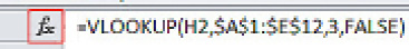
Figure 4-7
5. Edit the table_array part of the formula to reflect the new data range: $A$1:$E$13. You can do this either by changing the $E$12 to $E$13 or by reselecting the range to include $A$1:$E$13. To do this, click on the selection box next to Table_array in the Function Arguments dialog, as shown in Figure 4-8, and highlight the range $A$1:$E$13. Click on the selection box again to return to the main Vlookup() dialog box.
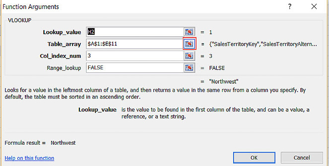
Figure 4-8
6. Click OK and copy down the formula to cell I12. You should now see Ireland in cell I11.
Note Even though the error showed up in cell I11, you begin the correction in cell I2 because you want to make sure the correction is applied to all the formulas, not just the one it shows up in.
Using the Table Feature to Solve the Missing Data Problem
However, it might be better to just get around this issue and resolve the problem permanently, particularly if the table_array part of the formula is regularly getting additions. To do this, you can convert a table array (where you will be pulling your matching data from) into a table. You’ve already seen tables in Chapter 2, but here’s a quick reminder:
1. Open the file 04_Vlookup_missing_data_table.
2. In the Sales Territories sheet, click on cell C8 and press Ctrl+T (or select Insert | Table).
3. In the Create Table dialog box that appears, make sure the My Table Has Headers box is checked and click OK.
4. Click anywhere in the table, click the Design tab, type Sales under Table Name, and press Enter to name the table Sales (see Figure 4-9).

Figure 4-9
5. Click in I2.
6. Follow the steps in the section “Situation 1: Matching Up Data in the Same Worksheet and File” to enter your Vlookup() function. (Note that you see one important difference: Your table_array part should now read Sales[#All] instead of A1:E12.)
7. In cell A13:E13, enter the following new territory:
|
12 |
12 |
Hungary |
Eastern Europe |
Europe |
8. In cell H13, type 12.
9. Copy down the formula from I2 to I13. Hungary now appears in cell I13, and you don’t have to make any changes to the table_array part of the formula.
Note Sometimes using a table makes cell references case-sensitive. I discovered (after checking at Experts Exchange) that you can do the following to fix this issue:
1. Choose File | Options.
2. In the Excel Options dialog that appears, scroll down the Advanced tab until you see Lotus Compatibility Settings For section and make sure the box Transition Formula Evaluation is unticked. You can see this in Figure 4-10.
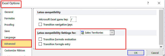
Figure 4-10
Handling Different Data Types
If the data types of the lookup value and the first column of a table array are not the same data type, you can end up with many many #N/A errors. This can happen, for example, if the first column of the table array is text and the lookup value is a number. You can see an example of this in the file 04_Text_and_numbers.
1. Highlight the range A3:A16 in the Text Part sheet and then look at the dropdown in the Number section of the Home tab. You can see that it is formatted as Text (see Figure 4-11).

Figure 4-11
2. Highlight the range A3:A16 in the Number Part sheet and then look at the dropdown in the Number section of the Home tab. You can see that it is formatted as Number (see Figure 4-12).

Figure 4-12
3. Look at the Vlookup() function in B3:B16 in the Number Part sheet. You can see that the function has returned #N/A errors, even though the Part Number entries look identical for both the entries in A3:A16 in the Number sheet and A3:A16 in the Text sheet.
4. Correct the #N/A errors by converting Part Number for both sheets to the same data type (e.g., Text or Number).
5. If step 4 doesn’t work, in the Text Part sheet, highlight the range A3:A16, click the yellow exclamation point, and choose Convert to Number (see Figure 4-13).
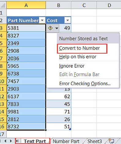
Figure 4-13
Removing Extra Spaces
Excel and all other programs (and computers themselves) see a space as a character, so one thing you might need to check is that you have the same number of spaces in both the lookup value and the matching entry in the first column of a table array.
If you don’t have the same number of spaces, you may have to use the Trim() function, which you have already seen in Chapter 2.
Fixing the Lookup Value When You Need to Pull in a Lot of Columns
Just a little while ago, I said that you need to copy in one set of data (i.e., SalesTerritoryRegion). But let’s say you have to copy in the data for SalesTerritoryCountry and SalesTerritoryGroup as well. Also assume that you need to work across two files, 04_Sales_territories and 04_Vlookup_functions_files. Of course, you could just enter the function again and again, but there’s another way:
1. Make sure the following files are open: 04_Sales_territories and 04_Vlookup_functions files.
2. If you have not done so already, in the 04_Vlookup_functions file, click in B2 and enter your Vlookup() formula to pull in SalesTerritoryRegion.
3. Go to the next heading by clicking in cell C2 and enter a Vlookup() function to pull in SalesTerritoryCountry.
4. In the 04_Vlookup_functions file, select Formulas | Lookup & Reference | VLOOKUP and then, in the Function Arguments dialog, when you have clicked in Lookup_value box and then clicked on A2, press F4 until you get the following configuration: $A2. (This fixes the column so that your Vlookup() will always refer to column A, but it allows the rows to change as the function is copied down. It also means that it is tethered to column A so that it’s always looking at column A as it is copied across.)
5. Copy across your Vlookup() to D2 (for SalesTerritoryGroup) and then amend your Vlookup() in D2 so the Col_index_num value is 4 instead of 3. It updates to show the correct value. (Note that when you check the function in C2, the Lookup_value still references column A.)
6. Repeat step 5 for SalesTerritoryAlternateKey but change the Col_index_num value to 5.
Note Of course, another tweak would be to add column numbers above your table array and refer to them in your Vlookup(). You can see an example of this in the file 04_Vlookup_function_column_with_numbers, which references 04_Sales_territories_with_numbers. Note how the column numbers have been entered into B1:E1 in the 04_Sales_territories_with_numbers file. You use these numbers instead of entering them into the Col_index_num part of the function. In this case, in the Col_index_num part of the Vlookup(), you enter the cell that has the column number (in the Sales territories with numbers file) but configure it (using F4) to show C$1.
|
Survival Tip If you open 04_Vlookup_function_column_with_numbers without having 04_Sales_territories_with_numbers open, you see REF! instead of the values. The good news is that when you open the file, the correct values appear. |
Using Vlookup() to Identify New Entries
One very common scenario is that product lists or nominal ledger codes are added from a previous month. When this happens, you need to identify what new entries you have that you didn’t have in the previous month.
1. Ensure that you have these two files open: 04_This_month_file and 04_Last_month_file.
2. In the 04_This_month_file workbook, add the new column heading Last Month in cell E1.
3. In cell E2, enter a Vlookup() that looks up the matching account number against the 04_Last_month_file workbook and returns the matching amount.
4. Click in E2 and select Formulas | Lookup & Reference | VLOOKUP.
5. Click on B2. [@Account] appears in the Lookup_value box in the Function Arguments dialog.
6. Click in the Table_array part of the Vlookup() function.
7. Go to the 04_Last_month file and highlight columns A to D. Note that Excel gives you the table reference '04_Last_month_file.xlsx'!Table1[#All].
8. Enter 4 in the Col_index_num box.
9. Enter FALSE for Range_lookup.
10. Click OK. Because the data is formatted as a table, it copies down automatically to the end of the range (row 642) in the 04_This_month_file.
11. Look at cells E641 and E642, and you see #N/A in both of them, indicating two new entries. The two new account entries in the 04_This_month file appear as #N/A because while they are account entries in the 04_This_month file, they are not entries in the 04_Last_month file. Because these are brand-new accounts (i.e., they did not exist in previous months), the best solution would be to add an Iferror() function around the Vlookup() that says “no match” or 0. This would make these new entries easier to identify.
Note You can find this completed file in 04_This_month_file_with_solution. It includes an Iferror() function to return 0 (zero) instead of #N/A.
Determining Whether You Need a Helper Cell and Adding One if You Do
To use a Vlookup() function, you need to have a matching column in both your lookup value and table array. You also need the lookup value to be a unique value.
In the examples in this chapter, you have had SalesTerritoryKey in both files. If you are using something like a barcode, that number will be both on your product and in the file with all the data you want to pull in. But that is not always the case. Let’s look at an example.
Say that you want to combine the quantity, price, invoice numbers, and product names for each of these products into one file. In one file, 04_FileA (see Table 4-1), you have the invoice number, product number, and quantity; this is on the sheet called 04_FileA. In the other file, 04_FileB (see Table 4-2), you have invoice number, product number, and product price.
Table 4-1: 04_FileA
|
Product Name |
Quantity |
|
|
100 |
A |
5000 |
|
100 |
C |
1000 |
|
200 |
A |
350 |
Table 4-2: 04_FileB
|
Product Name |
Price |
|
|
100 |
A |
200 |
|
100 |
B |
300 |
|
200 |
A |
500 |
What you want to do is link the two files together to get a total. However, neither the invoice number on its own nor the product number on its own is unique, so you can’t use a Vlookup() with the data as it is currently presented. So, what can you do?
The solution is to create a “helper cell” that will provide you with a unique identifier. You can create the unique identifier by using concatenation to combine the invoice number and the product name. This will be the field you then use to do the comparison.
You need to ensure that the helper cells are the same in both files and are the same data type (either text or numbers). You also need to make sure the helper cell is the first column in the table array part of the formula.
Follow these steps to create the helper cell:
1. In 04_FileA, click where you want the helper cell to go (to the left of the first column in cell A2) and type =.
2. Click in the first cell that contains text: B2 (i.e., the one that contains 100 in the Invoice Number column). Type &.
3. Click in cell C2 (i.e., the one that contains A in the Product Name column). You now have a formula that looks like this: =B2&C2.
4. Press Enter to copy down this formula (cell A2 should now read 100A) and to cells A3 and A4.
Note It can often be useful to give the helper cell columns the same name in both sheets.
You can see the solution for 04_FileA on the sheet called 04_FileASolution (see Table 4-3). In this case you used a helper cell (in cells E2:E4) to pull in the price from 04_FileB for the entries with the matching helper cell entry (Invoice Number and Product Name combined).
Table 4-3: 04_FileA (04_FileASolution Sheet)
|
Helper Cell |
Invoice |
Product |
Quantity |
Price |
|
100A |
100 |
A |
5000 |
200 |
|
100C |
100 |
C |
1000 |
300 |
|
200A |
200 |
A |
350 |
500 |
Repeat these steps to create a helper cell for 04_FileB. Table 4-4 shows the example in cell A2 of the 04_FileB_solution sheet. You now have a matching column, so you can use Vlookup() on this data. Check the formula in cell E2 of the 04_FileB_solution sheet to see how this Vlookup() works.
Table 4-4: 04_FileB (04_FileB_solution Sheet)
|
Helper Cell |
Invoice Number |
Product Name |
Price |
Quantity |
|
100A |
100 |
A |
200 |
5000 |
|
100C |
100 |
C |
300 |
1000 |
|
200A |
200 |
A |
500 |
350 |
Now you are familiar with the Vlookup() function. You have seen it in operation in three common situations: matching up data in the same worksheet and file, matching up data in the same file but different worksheets, and matching up data in two different files. You have also had a chance to explore and solve some of the most common problems that arise when using this powerful function, including what to do with different data types, how to clean up extra spaces, and how to fix a column so you can more easily copy the function across to other columns. You have also seen working examples of two common real-life situations: Pulling in matching data from a previous month and using a helper cell.