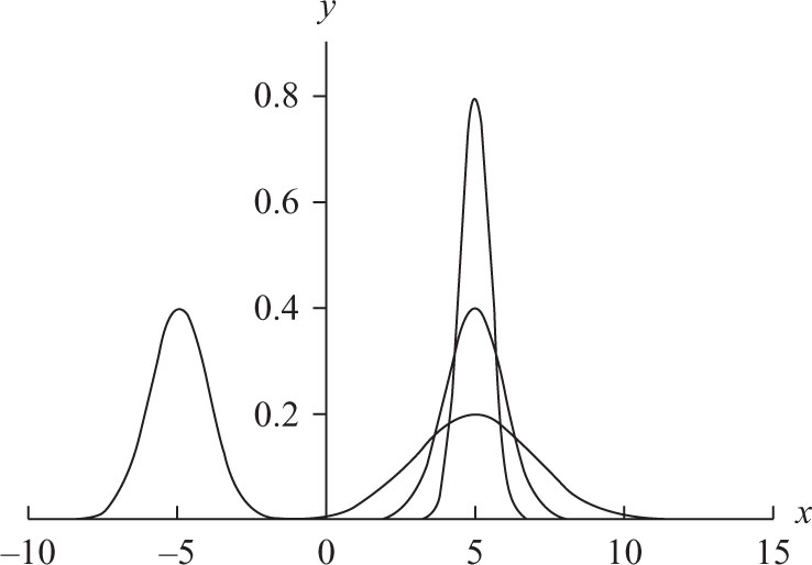
Statistics is the most widely applied of all mathematical disciplines and at the center of statistics lies the normal distribution, known to millions of people as the bell curve, or the bell-shaped curve. This is actually a two-parameter family of curves that are graphs of the equation
Several of these curves appear in Figure 8.1. Not only is the bell curve familiar to these millions, but they also know of its main use: to describe the general, or idealized, shape of graphs of data. It has, of course, many other uses and plays as significant a role in the social sciences as differentiation does in the natural sciences. As is the case with many important mathematical concepts, the rise of this curve to its current prominence makes for a tale that is both instructive and amusing. Actually, there are two tales here: the invention of the curve as a tool for computing probabilities and the recognition of its utility in describing data sets.
The origins of the mathematical theory of probability are justly attributed to the famous correspondence between Fermat and Pascal, which was instigated in 1654 by the queries of the gambling Chevalier de Mèrè. Among the various types of problems they considered were binomial distributions which today would be described by such sums as
that denotes the likelihood of between i and j successes in trials of probability p. As the examples they worked out involved only small values of n, they were not concerned with the computational challenge that the evaluation of sums of this type presents in general. However, more complicated computations were not long in coming. For example, in 1712 the Dutch mathematician’s Gravesande tested the hypothesis that male and female births are equally likely against the actual births in London over the 82 years 1629-1710 [14, 16]. He noted that the relative number of male births varies from alow of 7765/15,448 = 0.5027 in 1703 to a high of 4748/8855 = 0.5362 in 1661. ’s Gravesande multiplied these ratios by 11,429 – the average number of births over this 82 year span. These gave him nominal bounds of 5745 and 6128 on the number of male births in each year. Consequently, the probability that the observed excess of male births is due to randomness alone is the 82nd power of

’ s Gravesande did make use of the recursion

suggested by Newton for similar purposes, but even so this is clearly an onerous task. Since the probability of this difference in birth rates recurring 82 years in a row is the extremely small number 0.29282, ’s Gravesande drew the conclusion that the higher male birth rates were due to divine intervention.
In the following year, James and Nicholas Bernoulli found estimates for binomial sums of the type of (2). These estimates, however, did not involve the exponential function ex. De Moivre began his search for such approximations in 1721. In 1733, he proved that
and
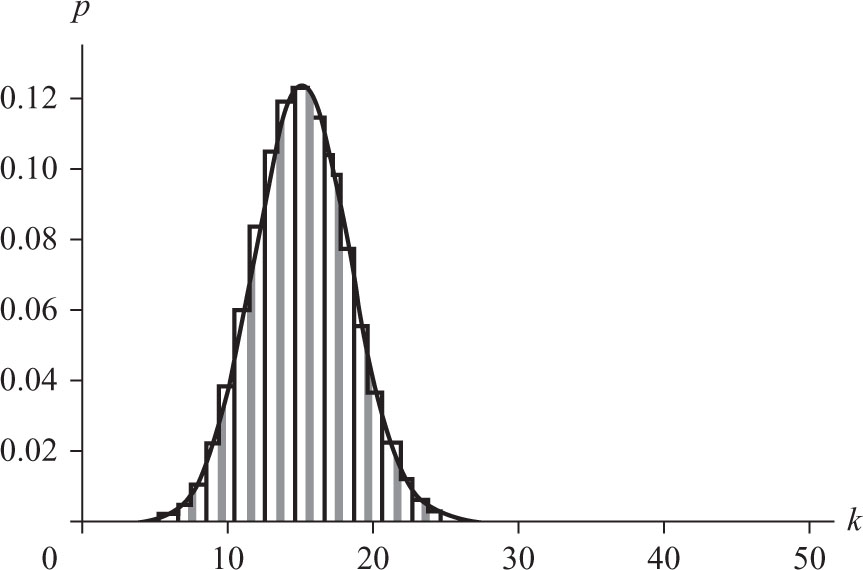
De Moivre also asserted that the above (4) could be generalized to a similar asymmetrical context. This is, of course, quite clear, and a proof is required only to clarify the precision of the approximation. Figure 8.2 demonstrates how the binomial probabilities associated with 50 independent repetitions of a Bernoulli trial with probability p = 0.3 of success are approximated by such an exponential curve. (A Bernoulli trial is the most elementary of all random experiments. It has two outcomes, usually termed success and failure.) De Moivre’s discovery is standard fare in all introductory statistics courses where it is called the normal approximation to the binomial and rephrased as
where

Since the above integral is easily evaluated by numerical methods and quite economically described by tables, it does indeed provide a very practical approximation for cumulative binomial probabilities.
Astronomy was the first science to call for accurate measurements. Consequently, it was also the first science to be troubled by measurement errors and to face the question of how to proceed in the presence of several distinct observations of the same quantity. In the 2nd century BCE Hipparchus seems to have favored the midrange. Ptolemy, in the 2nd century CE, when faced with several discrepant estimates of the length of a year, may have decided to work with the observation that best fit his theory [29]. Toward the end of the sixteenth century, Tycho Brahe incorporated the repetition of measurements into the methodology of astronomy. Curiously, he failed to specify how these repeated observations should be converted into a single number. Consequently, astronomers devised their own, often ad hoc, methods for extracting a mean, or data representative, out of their observations. Sometimes they averaged, sometimes they used the median, sometimes they grouped their data and resorted to both averages and medians. Sometimes they explained their procedures, but often they did not. Consider, for example, the following excerpt which comes from Kepler [19] and whose observations were, in fact, made by Brahe himself:
On 1600 January 13/23 at 11h 50m the right ascension of Mars was:
Kepler’s choice of data representative is baffling. Note that

and it is difficult to believe that an astronomer who recorded angles to the nearest second could fail to notice a discrepancy larger than a minute. The consensus is that the chosen mean could not have been the result of an error but must have been derived by some calculations. The literature contains at least two attempts to reconstruct these calculations but the author finds neither convincing, since both explanations are ad hoc, there is no evidence of either ever having been used elsewhere, and both result in estimates that differ from Kepler’s by at least five seconds.
To the extent that they recorded their computation of data representatives, the astronomers of the time seem to be using improvised procedures that had both averages and medians as their components [7, 29, 30]. The median versus average controversy lasted for several centuries and now appears to have been resolved in favor of the latter, particularly in scientific circles. As will be seen from the excerpts below, this decision had a strong bearing on the evolution of the normal distribution.
The first scientist to note in print that measurement errors are deserving of a systematic and scientific treatment was Galileo in his famous Dialogue Concerning the Two Chief Systems of the World – Ptolemaic and Copernican, published in 1632. His informal analysis of the properties of random errors inherent in the observations of celestial phenomena is summarized by S.M. Stigler, as:
1.There is only one number which gives the distance of the star from the center of the earth, the true distance.
2.All observations are encumbered with errors, due to the observer, the instruments, and the other observational conditions.
3.The observations are distributed symmetrically about the true value; that is the errors are distributed symmetrically about zero.
4.Small errors occur more frequently than large errors.
5.The calculated distance is a function of the direct angular observations such that small adjustments of the observations may result in a large adjustment of the distance.
Unfortunately, Galileo did not address the question of how the true distance should be estimated. He did, however, assert that: “… it is plausible that the observers are more likely to have erred little than much.” It is therefore not unreasonable to attribute to him the belief that the most likely true value is that which minimizes the sum of its deviations from the observed values. (That Galileo believed in the straightforward addition of deviations is supported by his calculations.) In other words, faced with the observed values x1, x2,…, xn, Galileo would probably have agreed that the most likely true value is the x that minimizes the function
As it happens, this minimum is well known to be the median of x1; x2,…, xn and not their average, a fact that Galileo was likely to have found quite interesting.
This is easily demonstrated by an inductive argument that is based on the observation that if these values are re-indexed so that x1 < x2 < … < xn, then

whereas

It took hundreds of years for the average to assume the near universality that it now possesses and its slow evolution is quite interesting. Circa 1660 we find Robert Boyle, later president of the Royal Society, arguing eloquently against the whole idea of repeated experiments:
… experiments ought to be estimated by their value, not their number;… a single experiment… may as well deserve an entire treatise …. As one of those large and orient pearls… may outvalue a very great number of those little… pearls, that are to be bought by the ounce …
In an article that was published posthumously in 1722, Roger Cotes made the following suggestion:
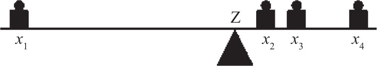
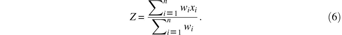
Let p be the place of some object defined by observation, q, r, s, the places of the same object from subsequent observations. Let there also be weights P, Q, R, S reciprocally proportional to the displacements which may arise from the errors in the single observations, and which are given from the given limits of error; and the weights P, Q, R, S are conceived as being placed at p, q, r, s, and their center of gravity Z is found: I say the point Z is the most probable place of the object, and may be safely had for its true place.
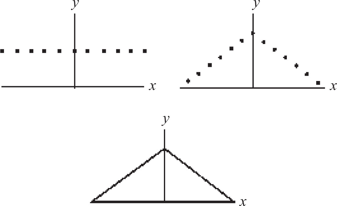
Cotes apparently visualized the observations as tokens x1; x2,…, xn (= p, q, r, s,…) with respective physical weights w1, w2,…, wn(= P, Q, R, S,…) lined up
on a horizontal axis (Figure 8.3 displays a case where n = 4 and all the tokens have equal weight). Having done this, it was natural for him to suggest that the center of gravity Z of this system should be designated to represent the observations. After all, in physics too, a body’s entire mass is assumed to be concentrated in its center of gravity and so it could be said that the totality of the body’s points are represented by that single point. That Cotes’s proposed center of gravity agrees with the weighted average can be argued as follows. By the definition of the center of gravity, if the axis is pivoted at Z it will balance and hence, by Archimedes’s law of the lever,

or
Of course, when the weights wi are all equal, Z becomes the classical average

It has been suggested that this is an early appearance of the method of least squares. In this context this method proposes that we represent the data x1, x2,…, xn by the x which minimizes the function
Differentiation with respect to x makes it clear that it is the Z of (6) that provides this minimum. Note that the median minimizes the function f(x) of (5) whereas the (weighted) average minimizer the function g(x) of (7). It is curious that each of the two foremost data representatives can be identified as the minimize of a nonobvious, though fairly natural, function. It is also frustrating that so little is known about the history of this observation.
Thomas Simpson’s paper of 1756 is of interest here for two reasons. First comes his opening paragraph:
It is well known to your Lordship, that the method practiced by astronomers, in order to diminish the errors arising from the imperfections of instruments, and of the organs of sense, by taking the Mean of several observations, has not been generally received, but that some persons, of considerable note, have been of opinion, and even publickly maintained, that one single observation, taken with due care, was as much to be relied on as the Mean of a great number.
Thus, even as late as the mid-18th century doubts persisted about the value of repetition of experiments. More important, however, was Simpson’s experimentation with specific error curves — probability densities that model the distribution of random errors. In the two propositions, Simpson computed the probability that the error in the mean of several observations does not exceed a given bound when the individual errors take on the values

with probabilities that are proportional to either

or

Simpson’s choice of error curves may seem strange, but they were in all likelihood dictated by the state of the art of probability at that time. For r = 1 these two distributions yield the two top graphs of Figure 8.4. One year later, Simpson, while effectively inventing the notion of a continuous error distribution, dealt with similar problems in the context of the error curves described in the bottom of Figure 8.4.
In 1774, Laplace proposed the first of his error curves. Denoting this function by ϕ(x), he stipulated that it must be symmetric in x, monotone decreasing for x > 0 and:
Now, as we have no reason to suppose a different law for the ordinates than for their differences, it follows that we must, subject to the rules of probabilities, suppose the ratio of two infinitely small consecutive differences to be equal to that of the corresponding ordinates. We thus will have

Therefore

… therefore

Laplace’s argument can be paraphrased as follows. Aside from their being symmetrical and descending (for x > 0), we know nothing about either ϕ(x) or ϕ′ (x). Hence, presumably by Occam’s razor, it must be assumed that they are proportional (the simpler assumption of equality leads to ϕ(x) = Ce|*|, which is impossible). The resulting differential equation is easily solved and the extracted error curve is displayed in Figure 8.5. There is no indication that Laplace was in any way disturbed by this curve’s nondifferentiability at x = 0. We are about to see that he was perfectly willing to entertain even more drastic singularities.
Laplace must have been aware of the shortcomings of his rationale, for three short years later he proposed an alternative curve. Let a be the supremum of all the possible errors (in the context of a specific experiment) and let n be a positive integer.
Choose n points at random within the unit interval, thereby dividing it into n + 1 spacings. Order the spacings as:

Let di be the expected value of di Draw the points (i/n, di), i= 1,2,…, n + 1 and let n become infinitely large. The limit configuration is a curve that is proportional to ln(a/x) on (0, a]. Symmetry and the requirement that the total probability must be 1 then yield Laplace’s second candidate for the error curve (Fig. 8.6):

This curve, with its infinite singularity at 0 and finite domain (a reversal of the properties of the error curve of Figure 8.5 and the bell-shaped curve), constitutes a step backward in the evolutionary process and one suspects that Laplace was seduced by the considerable mathematical intricacies of the curve’s derivation. So much so that he felt compelled to comment on the curve’s excessive complexity and to suggest that error analyses using this curve should be carried out only in “very delicate” investigations, such as the transit of Venus across the sun.
Shortly thereafter, in 1777, Daniel Bernoulli wrote:
Astronomers as a class are men of the most scrupulous sagacity; it is to them therefore that I choose to propound these doubts that I have sometimes entertained about the universally accepted rule for handling several slightly discrepant observations of the same event. By these rules the observations are added together and the sum divided by the number of observations; the quotient is then accepted as the true value of the required quantity, until better and more certain information is obtained. In this way, if the several observations can be considered as having, as it were, the same weight, the center of gravity is accepted as the true position of the object under investigation. This rule agrees with that used in the theory of probability when all errors of observation are considered equally likely. But is it right to hold that the several observations are of the same weight or moment or equally prone to any and every error? Are errors of some degrees as easy to make as others of as many minutes? Is there everywhere the same probability? Such an assertion would be quite absurd, which is undoubtedly the reason why astronomers prefer to reject completely observations which they judge to be too wide of the truth, while retaining the rest and, indeed, assigning to them the same reliability.
It is interesting to note that Bernoulli acknowledged averaging to be universally accepted. As for the elusive error curve, he took it for granted that it should have a finite domain and he was explicit about the tangent being horizontal at the maximum point and almost vertical near the boundaries of the domain. He suggested the semi-ellipse as such a curve, which, following a scaling argument, he then replaced with a semicircle.
The next important step has its roots in a celestial event that occurred on January 1,1801. On that day the Italian astronomer Giuseppe Piazzi sighted a heavenly body that he strongly suspected to be a new planet. He announced his discovery and named it Ceres. Unfortunately, six weeks later, before enough observations had been taken to make possible an accurate determination of its orbit, so as to ascertain that it was indeed a planet, Ceres disappeared behind the sun and was not expected to re-emerge for nearly a year. Interest in this possibly new planet was widespread and astronomers throughout Europe prepared themselves by compu-guessing the location where Ceres was most likely to reappear. The young Gauss, who had already made a name for himself as an extraordinary mathematician, proposed that an area of the sky be searched that was quite different from those suggested by the other astronomers and he turned out to be right.
Gauss explained that he used the least squares criterion to locate the orbit that best fit the observations. This criterion was justified by a theory of errors that was based on the following three assumptions:
1.Small errors are more likely than large errors.
2.For any real number ∊, the likelihood of errors of magnitudes ∊ and –∊ are equal.
3.In the presence of several measurements of the same quantity, the most likely value of the quantity being measured is their average.
On the basis of these assumptions he concluded that the probability density for the error (that is, the error curve) is

where h is a positive constant that Gauss thought of as the “precision of the measurement process.” We recognize this as the bell curve determined by μ = 0 and σ = 1/ h.
h.
Gauss’ s ingenious derivation of this error curve made use of only some basic probabilistic arguments and standard calculus facts. As it falls within the grasp of undergraduate mathematics majors with a course in calculus-based statistics, his proof is presented here with only minor modifications.
Let p be the true (but unknown) value of the measured quantity, let n independent observations yield the estimates M1, M2,…. Mn, and let ϕ(x) be the random error’s probability density function. Gauss took it for granted that this function is differentiable. Assumption 1 above implies that ϕ(x) has a maximum at x = 0 whereas Assumption 2 means that ϕ(-x)= ϕ(x). If we define

then

Note that Mi–p denotes the error of the ith measurement and consequently, since these measurements (and errors) are assumed to be stochastically independent, it follows that

is the joint density function for the $n$ errors. Gauss interpreted Assumption 3 as saying, in modern terminology, that

is the maximum likelihood estimate of p. In other words, given the measurements M1,M2,…, Mn the choice p = M maximizes the value of Ω. Hence,
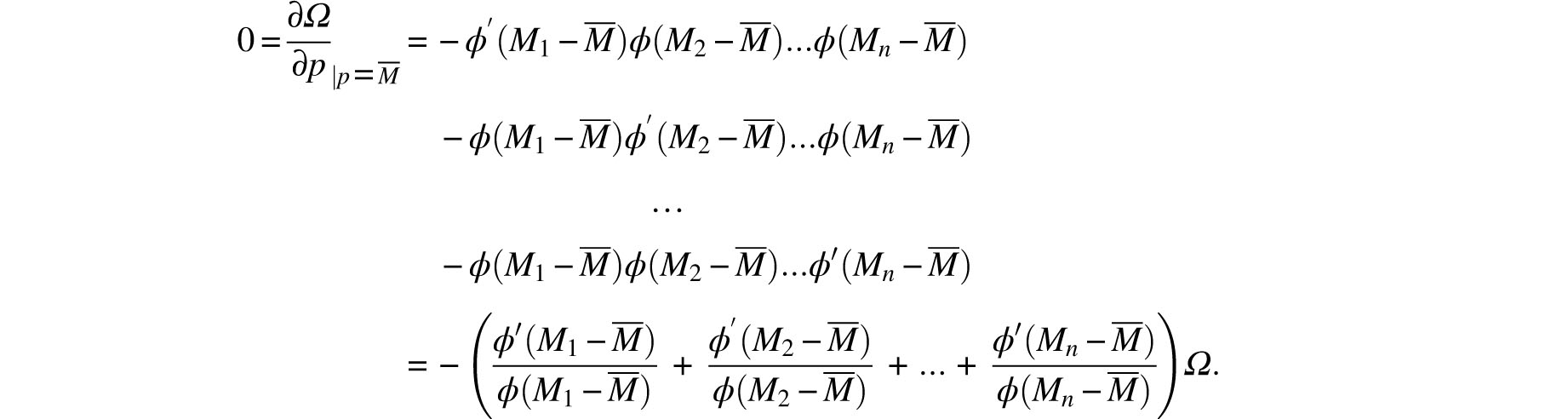
It follows that
Recall that the measurements Mi can assume arbitrary values and in particular, if M and N are arbitrary real numbers, we may use

for which set of measurements

Substitution into (8) yields

or

It is a well known exercise that this homogeneity condition, when combined with the continuity of f, implies that f(x)= kx for some real number k. This yields the differential equation

Integration with respect to x yields

In order for ϕ(x) to assume a maximum at x = 0, k must be negative and so we may set k/2 = −h2. Finally, since

it follows that

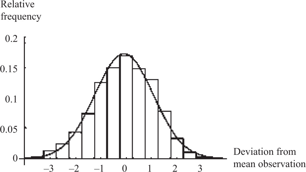
Figure 8.7 displays a histogram of some measurements of the right ascension of Mars, together with an approximating exponential curve. The fit is certainly striking.
It was noted above that the average is in fact a least squares estimator of the data. This means that Gauss used a particular least squares estimation to justify his theory of errors which in turn was used to justify the general least squares criterion. There is an element of boot-strapping in this reasoning that has left later statisticians dissatisfied and may have had a similar effect on Gauss himself. He returned to the subject twice, twelve and thirty years later, to explain his error curve by means of different chains of reasoning.
Actually, a highly plausible explanation is implicit in the Central Limit Theorem published by Laplace in 1810. Laplace’s translated and slightly paraphrased statement is:
… if it is assumed that for each observation the positive and negative errors are equally likely, the probability that the mean error of n observations will be contained within the bounds ±rh / n, equals

where h is the interval within which the errors of each observation can fall. If the probability of error
±x is designated by ϕ(x/h), then k is the integral 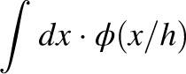 evaluated from
 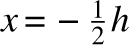 to
to 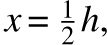 , and k’ is the integral
 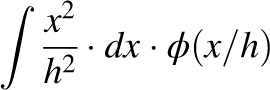 evaluated in the same interval.
Loosely speaking, Laplace’s theorem states that if the error curve of a single observation is symmetric, then the error curve of the sum of several observations is indeed approximated by one of the Gaussian curves. Hence if we take the further step of imagining that the error involved in an individual observation is the aggregate of a large number of “elementary” or “atomic” errors, then this theorem predicts that the random error that occurs in that individual observation is indeed controlled by De Moivre and Gauss’s curve.
This assumption, promulgated by Hagen and Bessel, became known as the hypothesis of elementary errors. A supporting study had already been carried out by Daniel Bernoulli in 1780, albeit one of much narrower scope. Assuming a fixed error ±α for each oscillation of a pendulum clock, Bernoulli concluded that the accumulated error over, say, a day would be, in modern terminology, approximately normally distributed.
This might be the time to recapitulate the average’s rise to the prominence it now enjoys as the estimator of choice. Kepler’s treatment of his observations shows that around 1600 there still was no standard procedure for summarizing multiple observations. Around 1660 Boyle still objected to the idea of combining several measurements into a single one. Half a century later, Cotes proposed the average as the best estimator. Simpson’s article of 1756 indicates that the opponents of the process of averaging, while apparently a minority, had still not given up. Bernoulli’s article of 1777 admitted that the custom of averaging had become universal. Finally, some time in the first decade of the 19th century, Gauss assumed the optimality of the average as an axiom for the purpose of determining the distribution of measurement errors.
The first mathematician to extend the provenance of the normal distribution beyond the distribution of measurement errors was Adolphe Quetelet (1796–1874). He began his career as an astronomer but then moved on to the social sciences. Consequently, he possessed an unusual combination of qualifications that placed him in just the right position for him to be able to make one of the most influential scientific observations of all times.
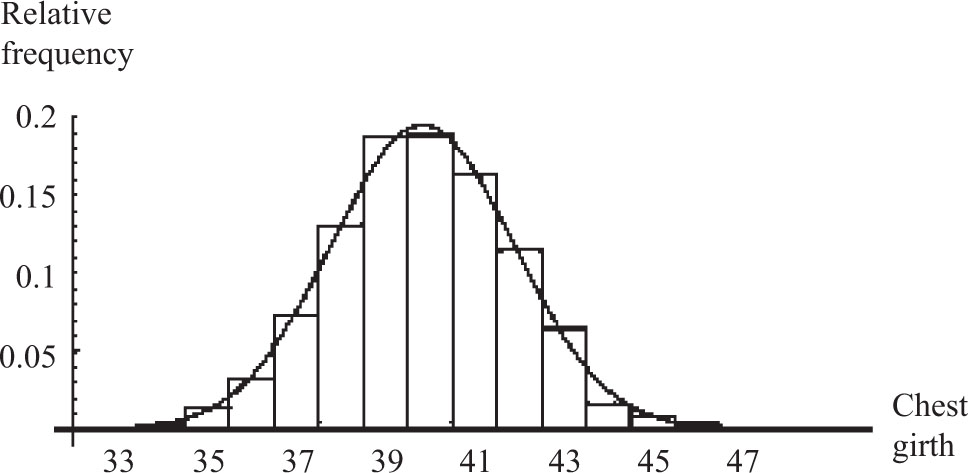
In his 1846 book Letters addressed to H. R. H. the grand duke of Saxe Coburg and Gotha, on the Theory of Probabilities as Applied to the Moral and Political Sciences, Quetelet extracted the contents of Table 1 from the Edinburgh Medical and Surgical Journal (1817) and contended that the pattern followed by the variety of its chest measurements was identical with that formed by the type of repeated measurements that are so common in astronomy. In modern terminology, Quetelet claimed that the chest measurements of Table 1 were normally distributed. The readers are left to draw their own conclusions regarding the closeness of the fit attempted in Figure 8. The more formal χ2 normality test yields a  value of 47.1, which is much larger than the cutoff value of
 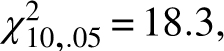 meaning that by modern standards these data cannot be viewed as being normally distributed. This discrepancy indicates that Quetelet’s justification of his claim of the normality the chest measurements merits a substantial dose of skepticism. It appears here in translation:
| Girth | Frequency |
| 33 | 3 |
| 34 | 18 |
| 35 | 81 |
| 36 | 185 |
| 37 | 420 |
| 38 | 749 |
| 39 | 1,073 |
| 40 | 1,079 |
| 41 | 934 |
| 42 | 658 |
| 43 | 370 |
| 44 | 92 |
| 45 | 50 |
| 46 | 21 |
| 47 | 4 |
| 48 | 1 |
| 5,738 |
Table 8.1: Chest measurements of Scottish soldiers.
I now ask if it would be exaggerating, to make an even wager, that a person little practiced in measuring the human body would make a mistake of an inch in measuring a chest of more than 40 inches in circumference? Well, admitting this probable error, 5,738 measurements made on one individual would certainly not group themselves with more regularity, as to the order of magnitude, than the 5,738 measurements made on the scotch [sic] soldiers; and if the two series were given to us without their being particularly designated, we should be much embarrassed to state which series was taken from 5,738 different soldiers, and which was obtained from one individual with less skill and ruder means of appreciation.
This argument, too, is unconvincing. It would have to be a strange person indeed who could produce results that diverge by 15” while measuring a chest of girth 40”. Any idiosyncrasy or unusual conditions (fatigue, for example) that would produce such unreasonable girths is more than likely to skew the entire measurement process to the point that the data would fail to be normal.
It is of interest to note that Quetelet was the man who coined the phrase the average man. In fact, he went so far as to view this mythical being as an ideal form whose various corporeal manifestations were to be construed as measurements that are beset with errors:
If the average man were completely determined, we might … consider him as the type of perfection; and everything differing from his proportions or condition, would constitute deformity and disease; everything found dissimilar, not only as regarded proportion or form, but as exceeding the observed limits, would constitute a monstrosity.
Quetelet was quite explicit about the application of this, now discredited, principle to the Scottish soldiers. He takes the liberty of viewing the measurements of the soldiers’ chests as a repeated estimation of the chest of the average soldier:
I will astonish you in saying that the experiment has been done. Yes, truly, more than a thousand copies of a statue have been measured, and though I will not assert it to be that of the Gladiator, it differs, in any event, only slightly from it: these copies were even living ones, so that the measures were taken with all possible chances of error, I will add, moreover, that the copies were subject to deformity by a host of accidental causes. One may expect to find here a considerable probable error.
Finally, it should be noted that Table 1 contains substantial errors. The original data was split amongst tables for eleven local militias, cross-classified by height and chest girth, with no marginal totals, and Quetelet made numerous mistakes in extracting his data. The actual counts are displayed in Table 2 where they are compared to Quetelet’s counts.
Quetelet’s book was very favorably reviewed in 1850 by the eminent and eclectic British scientist John F. W. Herschel [18]. This extensive review contained the outline of a different derivation of Gauss’s error curve, which begins with the following three assumptions:
1.… the probability of the concurrence of two or more independent simple events is the product of the probabilities of its constituents considered singly;
2.… the greater the error the less its probability …
3.… errors are equally probable if equal in numerical amount …
Herschel’s third postulate is much stronger than the superficially similar symmetry assumption of Galileo and Gauss. The latter is one-dimensional and is formalized as ϕ(∊) = ϕ (− ∊) whereas the former is multi-dimensional and is formalized as asserting the existence of a function ψ such that
| Girth | Actual Frequency | Quetelet’s Frequency |
| 33 | 3 | 3 |
| 34 | 19 | 18 |
| 35 | 81 | 81 |
| 36 | 189 | 185 |
| 37 | 409 | 420 |
| 38 | 753 | 749 |
| 39 | 1,062 | 1,073 |
| 40 | 1,082 | 1,079 |
| 41 | 935 | 934 |
| 42 | 646 | 658 |
| 43 | 313 | 370 |
| 44 | 168 | 92 |
| 45 | 50 | 50 |
| 46 | 18 | 21 |
| 47 | 3 | 4 |
| 48 | 1 | 1 |
| 5,738 | 5,732 |
Table 8.2: Chest measurements of Scottish soldiers.
Essentially the same derivation had already been published by the American R. Adrain in 1808, prior to the publication of but subsequent to the location of Ceres. In his 1860 paper on the kinetic theory of gases, the renowned British physicist J. C. Maxwell repeated the same argument and used it, in his words:
To find the average number of particles whose velocities lie between given limits, after a great number of collisions among a great number of equal particles.
The social sciences were not slow to realize the value of Quetelet’s discovery to their respective fields. The American Benjamin A. Gould, the Italians M. L. Bodio and Luigi Perozzo, the Englishman Samuel Brown, and the German Wilhelm Lexis all endorsed it. Most notable amongst its proponents was the English gentleman and scholar Sir Francis Galton who continued to advocate it over the span of several decades. This aspect of his career began with his 1869 book Hereditary Genius in which he sought to prove that genius runs in families. As he was aware that exceptions to this rule abound, it had to be verified as a statistical, rather than absolute, truth. What was needed was an efficient quantitative tool for describing populations and that was provided by Quetelet whose claims of the wide ranging applicability of Gauss’s error curve Galton had encountered and adopted in 1863.
As the description of the precise use that Galton made of the normal curve would take us too far afield, we shall only discuss his explanation for the ubiquity of the normal distribution. In his words:
Considering the importance of the results which admit of being derived whenever the law of frequency of error can be shown to apply, I will give some reasons why its applicability is more general than might have been expected from the highly artificial hypotheses upon which the law is based. It will be remembered that these are to the effect that individual errors of observation, or individual differences in objects belonging to the same generic group, are entirely due to the aggregate action of variable influences in different combinations, and that these influences must be.
1.all independent in their effects,
2.all equal,
3.all admitting of being treated as simple alternatives “above average” or “below average,”
4.the usual tables are calculated on the further supposition that the variable influences are infinitely numerous.
This is, of course, an informal restatement of Laplace’s Central Limit Theorem. The same argument had been advanced by Herschel. Galton was fully aware that conditions (1–4) never actually occur in nature and tried to show that they were unnecessary. His argument, however, was vague and inadequate. Over the past two centuries the Central Limit Theorem has been greatly generalized and a newer version, known as Lindeberg’s Theorem, exists which makes it possible to dispense with requirement (2). Thus, De Moivre’s curve (1) emerges as the limiting, observable distribution even when the aggregated “atoms” possess a variety of nonidentical distributions. In general it seems to be commonplace for statisticians to attribute the great success of the normal distribution to these generalized versions of the Central Limit Theorem. Quetelet’s belief that all deviations from the mean were to be regarded as errors in a process that seeks to replicate a certain ideal has been relegated to the same dustbin that contains the phlogiston and aether theories.
A word must be said about the origin of the term normal. Its aptness is attested by the fact that three scientists independently initiated its use to describe the error curve

These were the American C. S. Peirce in 1873, the Englishman Sir Francis Galton in 1879, and the German Wilhelm Lexis, also in 1879. Its widespread use is probably due to the influence of the great statistician Karl E. Pearson, who had this to say in 1920:
Many years ago [in 1893] I called the Laplace-Gaussian curve the normal curve, which name, while it avoids the international question of priority, has the disadvantage of leading people to believe that all other distributions of frequency are in one sense or another abnormal.
At first it was customary to refer to Gauss’s error curve as the Gaussian curve and Pearson, unaware of De Moivre’s work, was trying to reserve some of the credit of discovery to Laplace. By the time he realized his error the normal curve had become one of the most widely applied of all mathematical tools and nothing could have changed its name. It is quite appropriate that the name of the error curve should be based on a misconception.
The author thanks his colleagues James Church and Ben Cobb for their helpfulness, Martha Siegel for her encouragement, the editor Frank A. Farris and the anonymous referees for their constructive critiques.