5.1 Introduction
Pain is distinguished by duration as acute (less than 6 weeks), subacute (6–12 weeks), and chronic (12 weeks or more) pain. Approximately 100 million US adults suffer from common chronic pain conditions, more than the number affected by heart disease, diabetes, and cancer combined [1]. The economic cost of chronic pain in adults, including health care expenses and lost productivity, is $560–630 billion annually [1]. Seven in ten Americans feel that pain research and management should be one of the medical community’s top few priorities (16%) or a high priority (55%) [2].
One form of chronic pain is nociceptive pain, which is the normal response to injury of tissues such as muscles, visceral organs, joints, or bones. Another form is neuropathic pain, which involves dysfunction of (i) the peripheral nervous system (PNS) or (ii) the central nervous system (CNS). The latter case is amplification and generation of pain within the CNS itself due to distorted sensory processing, malfunctioning of pain-inhibitory mechanisms, and enhancing pain-facilitatory mechanisms [3–6]. An example is psychogenic pain, which does not usually have a physical origin [7, 8]. Highly prevalent symptoms in chronic pain are depression and anxiety [7–11], which are reported by more than 50% of patients with chronic pain [9]. Pain and depression may create a vicious cycle in which pain worsens depression and vice versa [10].
Low back pain, either acute or chronic, dominates other pain types [7] and affects about 80–84% of the population at least once at some point in life [12–14]. In the US Armed Services alone, low back pain was the primary diagnosis for more than seven million ambulatory care visits between 2000 and 2009 [15]. Current estimates are that approximately 25% of people with acute low back pain experience recurrent episodes, while 7–10% progress to a chronic state [15] and can experience significant physical, psychological, and social sequelae that affect their long-term functioning and quality of life [16]. According to [11], 70% of subjects with chronic low back pain report fatigue and 18% report depression. According to [17], 59% of the patients with chronic low back pain report poor sleep.
Chronic low back pain accounts for 22% of all chronic pain cases and for 35% of most persistent pain sites [7]. The classification of low back pain is complicated by the varying presentation and complex nature of pain [14]. The most common diffuse neuropathic pain without radiating beyond the buttocks is classified as nonspecific low back pain [14], which makes up 60% of individuals suffering from chronic low back pain [18].
The initial treatment for acute nonspecific low back pain is conservative, including nonopioid analgesics (acetaminophen, aspirin), nonsteroidal anti-inflammatory drugs (ibuprofen, ketoprofen), physiotherapy, dynamic strengthening exercises, thermotherapy, and, if necessary, a short course of muscle relaxants [13, 14]. Further, conservative methods include traction treatment, manual therapy, and transcutaneous electrical nerve stimulation (TENS) [14]. A commonly prescribed treatment for chronic pain is opioids (codeine, oxycodone, hydrocodone, and morphine) [13, 19]. The use of opioids is controversial due to severe addiction and misuse [13, 15, 16, 20, 21]. It is argued that chronic use of opioids is detrimental to people with back pain because they can aggravate depression, leading to a worsening of the pain [13]. Whenever possible, opioid medications in chronic noncancer pain should be avoided [20].
TENS is a common drug-free alternative treatment technique that stimulates selected sensory nerves and muscles via electrodes placed on the skin over the painful area [22–28]. The electrodes inject electric currents and, most importantly, electric fields into body. The theory is that the local electric field stimulation can modify both cause and perception of chronic pain. A number of systematic reviews of the effect of TENS on various painful conditions, such as labor pain, rheumatoid arthritis, phantom limb pain, and chronic lower back pain, are available [22, 24–28]. However, these reviews indicate that most controlled randomized clinical trials failed to show significant effects of the existing small-scale TENS systems with a strongly localized electric field distribution.
This design-based study is driven by the limitations of TENS. We introduce a conceptually different electromagnetic stimulation device. Instead of local high-intensity and suprathreshold TENS, we suggest to stimulate the PNS and muscular system of the entire lower body in a noncontact, patient-friendly way. At the same time, we suggest to use low or subthreshold power levels. In other words, we propose mild yet more broad electromagnetic treatment, potentially beneficial for nonspecific chronic pain. The proposed device [29, 30] would primarily affect peripheral nerves, the spinal cord, muscles, joints, and bone. Simultaneously, it could influence the somatosensory cortex via many affected pathways, in line with the modern concept of central control of pain [8]. Based on the numbers cited above [7, 14, 18], we can estimate that some 14% of all chronic pain cases might be subject to the proposed alternative treatment.
The text is organized as follows. Section 5.2 describes a theoretical device model, specifies the field distribution within the resonator, and describes hardware design, test, and functionality, including semiautomatic operation/tuning and representative continuous run times. Section 5.3 provides computational results for the electric field distribution within the body obtained via two independent numerical methods. Section 5.4 discusses possible device modifications, as well as potential application scenarios. Section 5.5 concludes the chapter.
5.2 Materials and Methods
5.2.1 Suprathreshold Versus Subthreshold Stimulation
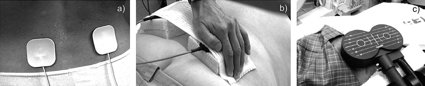
(a) Portable pulsed-current TENS (or PEMF) device from National Health Service (NHS) England website [32]. (b) Stationary continuous-current TENS device with sponge electrodes for low back pain treatment in Hannover, Germany [33]. (c) Induction coil-based peripheral neuropathic pain stimulation for low back pain treatment [34, 35]
Alternatively, a continuous current injection with a more powerful stationary device may be employed by chiropractors as shown in Fig. 5.1b [33]. When connected to the lower back, it creates a rather strong burning sensation. The electric field may also be injected via a noncontact induction coil [34, 35] as in Fig. 5.1c. Although a broader coverage with many electrodes is now possible, local suprathreshold effects still dominate.
With respect to treatment-persistent depression, only three nonpharmacological therapies have been approved by the FDA to date; all of them are electromagnetic and suprathreshold: transcranial magnetic stimulation [36], vagus nerve stimulation [37], and electroconvulsive therapy [38].
Subthreshold refers to a low-power electromagnetic stimulation that is too small to elicit action potentials. However, it still alters the axonal membrane potential [39]. This effect accumulates and maximizes toward axon terminals, i.e., synapses [39]. It is synaptic efficacy (or natural neurotransmission efficacy) that is altered and enhanced by the subthreshold stimulation [39]. In a chain of neurons, this stimulation could cause an incremental relay effect, which may further enhance neuronal network activity [39]. The theory of subthreshold stimulation [39–42] has been developed in application to transcranial current stimulation [39–47]. Low-field magnetic stimulation of depression is an active area of research [48–54]. The subthreshold technique is also a modern research direction in spinal cord stimulation [55–59], as it eliminates noxious and off-target paresthesia, while being efficient, as well as in vagus [60], occipital [61], proximal [62], and parasympathetic [63] nerve stimulation, and in neuromuscular stimulation [64]. Electrocutaneous subthreshold stimulation has been found to improve sleep and reduce reactive anxiety/depression [65].
5.2.2 Concept of the Magnetic Stimulator. Two-Dimensional Analytical Solution for Solenoidal E-Field
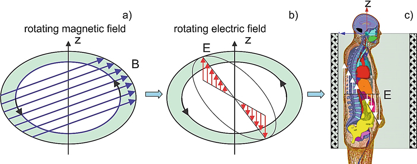
Concept of non-invasive electric field excitation via the induction mechanism. A rotating magnetic field shown in (a) excites the rotating electric field within the conductor (b) and within the body (c), respectively

The rotational character of the field also assures that not only one body cross section (e.g., coronal or sagittal) will be subject to the electric field excitation, but the entire body volume.
In the ideal, two-dimensional case and for any conducting target with a strict cylindrical symmetry placed into the device, either homogeneous or not, the corresponding two-dimensional problem, shown in Fig. 5.2a, b, will have an exact analytical solution in the quasi-static (or eddy current) approximation. The electric field within the target is given by [66].


5.2.3 Three-Dimensional Coil Resonator Design. Solenoidal E-Field
The external rotating magnetic flux density B is created using a volumetric resonator in the form of a low-pass birdcage coil. Resonators of this type (called “birdcage coils”) are routinely used as MRI radio frequency (RF) coils [67, 68], but for a completely different purpose, namely atomic spin excitation and RF signal acquisition. The resonant frequency in this application is very high, typically 64 MHz (for 1.5 T magnets) or higher. For our purpose, we decided to reconstruct that design for a much lower frequency band of 100 kHz or less. In particular, the band of 10 kHz has recently demonstrated great promise for spinal cord stimulation for back and leg chronic pain management [55–59, 69–77] with and without previous back surgeries [70, 72], and is utilized by TENS [78]. In addition to superior pain relief, the 10 kHz band may provide long-term improvements in quality of life and functionality for subjects with chronic low back and leg pain [77]. On the other hand, a wider band of 4–30 kHz has been used for polyneuropathy (a general degeneration of peripheral nerves that spreads toward the center of the body) electrostimulation treatment [79–82].
We chose the birdcage coil because it can produce a very homogeneous B-field in the transverse plane, and because it can produce a circularly polarized B-field. These features relax the requirements for accurate patient positioning relative to the coil. The patient has significant freedom of movement transversely within the coil, including freedom of rotation (thanks to circular polarization). This should enhance patient comfort and permit long treatment sessions.
The resonator concept will allow for an arbitrary “tonic” modulation [30] of the carrier frequency, which was found to beneficially address the variable nature of chronic pain across different patients [76]. This modulation can be either open- or closed-loop (e.g., a single-channel EEG signal fed back to the modulator).
When the resonant frequency becomes low as in the present case, the standard RF birdcage coil will possess very low inductance L. Tuning such a coil toward resonance at low frequencies would require large capacitance C. This, however, means a low Q-factor (quality factor  is the “gain” of the series resonator) and higher costs, as well as higher fabrication complexity [83, 84], and will restrict the use of the conventional birdcage coil to frequencies above at least a few megahertz. Different methods to overcome this difficulty have been suggested [83–88], but they are all limited to small-size coils.
To distribute the required capacitors uniformly around the coil circumference
To improve the mechanical stiffness of this self-supporting coil structure
To reduce rung tube diameter, simplifying assembly
To facilitate direct drive of the coil at a single rung (for each mode). The equivalent parallel resistance at resonance was significantly above 50 ohms for the 144 rung configuration, permitting the use of capacitive-only matching networks. Later in the development process, we decided not to use direct drive, but the option remains
However, we are not claiming that the particular number of rungs we used is optimal. All the coil geometrical parameters (number of rungs, rung and end ring tube diameters, coil length and diameter) are subject to optimization during design and construction of the next prototype. We may even consider switching to a fundamentally different coil winding design, such a saddle coil. That said, any optimization is not expected to dramatically improve the coil’s B-field. Improvements up to 20% may be possible (slightly more if the coil is made smaller).
Along with this, we employ carefully designed inductive power coupling. The inductive coupling blocks DC and acts as a balun (balanced-unbalanced transformer). This is useful in terms of both circuit design (we avoid having to install a transformer) and safety concerns (no direct path from the AC to the coil). It also allows adjusting the load resistance at resonance. Inductive coupling perturbs the current distribution in the coil significantly less than directly driving an individual rung. As a result, the resonator possesses a superior quality factor of approximately 300 [30]. Therefore, we may achieve any desired electric field levels of up to 50–100 V/m within the lower body due to the resonance effect and still use standard power electronics equipment.
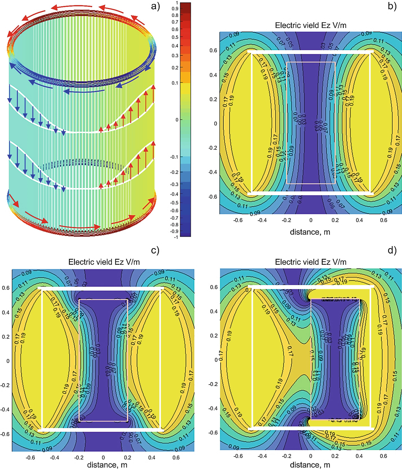
Current distribution in the coil resonator and the associated solenoidal electric field created by the coil when the ring current amplitude is 1 A for one resonant mode. (a) Electric current distribution in the coil along with the current color bar to scale; (b) Magnitude of the vertical electric field Ez in V/m for an empty coil in the coronal plane; (c) Magnitude of the vertical electric field Ez in V/m for the coil with a coaxial conducting cylinder 0.4 × 1 m inside; (d) Magnitude of the vertical electric field Ez in V/m for the coil with a conducting cylinder 0.4 × 1 m shifted in the transverse plane inside
From the modeling point of view, the resonant electric current in both rings at any fixed time instant behaves like a full period of a sine function of polar angle φ. This ring current distribution is shown in Fig. 5.3a. As time progresses, the ring current distribution shown in Fig. 5.3a rotates with angular frequency ω. As a result, the time-domain ring current i(t, φ) in the top and bottom rings can be expressed in the form


The useful current, which creates a nearly constant horizontal rotating magnetic field Br with amplitude B0 and axial rotating electric field Ez according to Eq. (5.2), is the rung current density j(t, φ). Contributions of each rung add up in a constructive manner. The ring current, on the other hand, does not contribute to the axial (or vertical) electric field, Ez. However, it may create a strong transverse electric field very close to the rings.
It should be pointed out that Eqs. (5.4) and (5.5) describe the rotating current behavior, which is a combination of two elementary resonant modes. Each elementary mode does not rotate and appears as depicted in Fig. 5.3a. However, when excited in quadrature (with a 90 degree phase shift and a 90 degree excitation offset along the coil circumference), both modes combine to create the current distribution given by Eqs. (5.4) and (5.5) and the associated rotating electric field. The rotation phenomenon enables us to treat the entire body and not merely a singular component or region.
5.2.4 Solenoidal Electric Field Distribution with and without a Simple Conducting Object
Figure 5.3b–d shows the resulting electric field distribution in the coil (coronal plane) when the current amplitude I0 = 1 ampere in either ring given by Eq. (5.4). The results are given for one resonant mode, as shown in Fig. 5.3a. Due to linearity, this result can simply be scaled for other excitation levels. Accurate field computations have been performed with the fast multipole method described in [89]. The magnitude of the axial component Ez in V/m for an empty coil is shown in Fig. 5.3b. The electric field is indeed zero at the coil’s center.
When a conducting object representing a load is inserted into the coil, the field distribution changes. Figure 5.3c shows the distribution when a conducting cylinder with a diameter of 0.4 m and a length of 1 m is inserted into the coil along its axis. The particular conductivity value σ does not matter since only the conductivity contrast, (σ − σair)/(σ + σair), is present in the solution [66]. This value is always unity since σair = 0.
An interesting and useful effect is observed in Fig. 5.3c: we see a “pulling” of the electric field into the cylinder close to the coil center. This is due to surface charges that appear at and near the cylinder tips. As a result, the electric field close to the cylinder surface at the center plane of the coil increases by nearly 36%.
Another remarkable observation (this effect is common in MRI RF coils) follows from Fig. 5.3d where the conducting cylinder has been shifted from the coil axis to the right by 0.2 m. While the electric field outside the conducting cylinder clearly changes, the field within the cylinder remains nearly the same, as observed in Fig. 5.3c. This may be explained as a result of the electric field being induced by the magnetic field, similar to eddy currents. Since the magnetic field is relatively homogeneous in the transverse plane of the coil, the induced electric fields in a load should not strongly depend on the transverse position of the load within the coil.
These rudimentary simulations allow us to establish two basic facts relevant for the analysis of realistic electric field distributions in a human body within the coil. First, we expect that the average transcutaneous electric field will be slightly higher than predicted by the air-filled coil model in dorsal, abdominal, and lumbar body regions. Second, we expect that the field within the body will not change significantly when the body is moved within the coil in the transverse plane; this circumstance seems to be useful from a practical point of view.
5.2.5 Contribution of Unpaired Electric Charges
Generally, the total electric field within the coil is expressed in terms of two auxiliary potentials. Instead of Eq. (5.1), one has

 is neglected (which gives us the Coulomb gauge, ∇ · A = 0), while it is still kept in Eq. (5.6). As a result, the − ∇ φ term in Eq. (5.6) becomes a conservative electric field contribution due to charge density alone, while the −∂A/∂t term is a true solenoidal electric field contribution due to current density alone.
In accordance with the (quasi)electrostatic theory [90], the conservative electric field is blocked by charges induced on a surface of a conducting object and does not penetrate into the object. Therefore, its contribution is ignored in the present study, similar to the theoretical models of transcranial magnetic stimulation or TMS. Note that this charge contribution may be quite large in the present problem, close to the bridging capacitors.
We have also performed full-wave ANSYS ED simulations of this coil and found that the capacitor voltage drop E-field does not significantly affect the E-field within the patient. The externally applied conservative E-field is expelled from the patient by the high conductivity of tissues. Only the E-field induced from the B-field is important.
5.2.6 Power Amplifier/Driver
In order to create the rotating magnetic and electric fields, as seen in Figs. 5.2a, b, two resonant modes are excited in the coil resonator. These modes display the same current distribution as shown in Fig. 5.3a, but rotated by 90 degrees about the coil axis with respect to each other as well as having an additional temporal phase shift of 90 degrees.
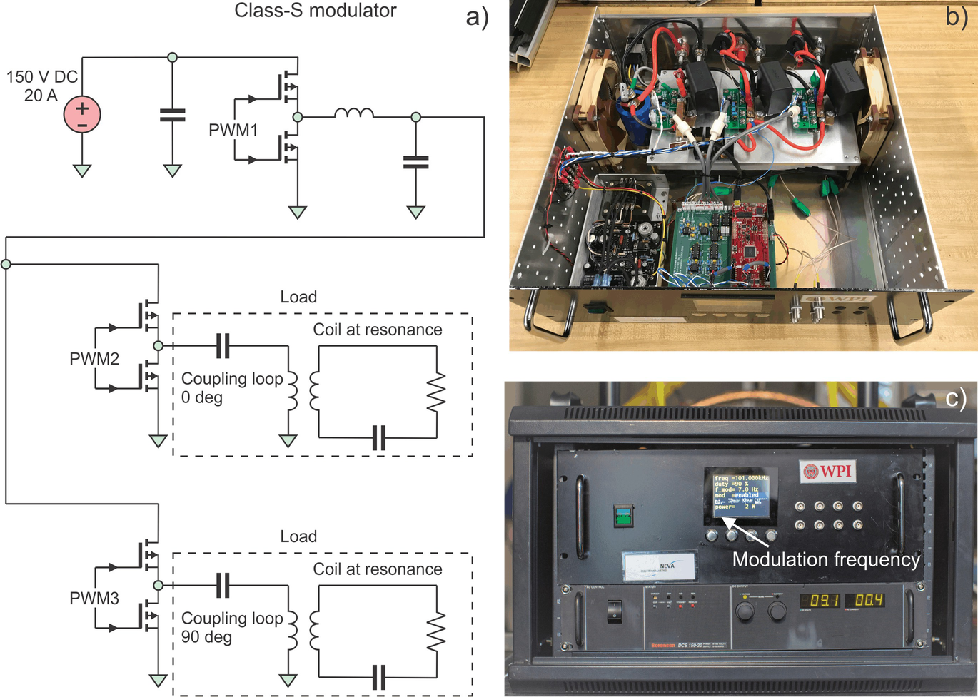
(a) High-level circuit schematic of the two-channel power amplifier. (b) Rackmount air-cooled assembly of the electronic hardware. (c) Amplifier display controlling output power and modulation frequency (if used)
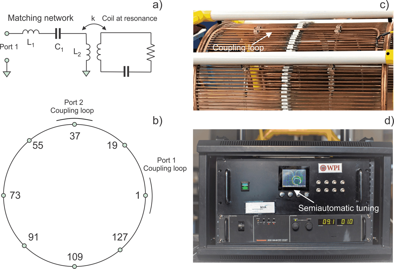
(a) Matching and tuning network of the power amplifier. (b) Assembly of two coupling-loop feed around the coil circumference with 144 rungs. (c) Noncontact inductive coupling of the power amplifier to the coil resonator at one port. (d) Smith chart/reflection coefficient display of the power amplifier controller used for semiautomatic tuning at any desired time instant
The PA output stage is powered by a 3 kW Sorensen DCS 150–20 Variable Regulated DC (direct current) power supply seen at the bottom of Fig. 5.4c. When connected to a standard three-phase 208 VAC outlet, the max RF output power is about 2.9 kW, based on 3 kW DC power. Alternatively, when connected into a single-phase 240 VAC outlet, the max RF power reduces to about 2.3 kW based on 2.4 kW DC power.
Arbitrary modulation (pulse or CW) of the carrier signal with a maximum modulation frequency component of 1 kHz is available via the modulator. The modulation bandwidth is limited mainly by the coil envelope time constant of about 1 ms. Typical modulation is sinusoidal in the 0.5–100 Hz range, generated by the PA firmware.
The PA also monitors its output power and load impedance. It uses this information to automatically adjust the carrier frequency in a narrow band such that the output power remains on target. The amplifier cost, including the DC power supply, is under $10,000. The prototype 100 kHz PA was assembled in a rackmount case shown in Figs. 5.4b, c.
The reason for designing a custom, fixed-frequency PA is the lack of an affordable and appropriate commercial model. Industrial low-frequency RF power supplies, e.g., Comdel’s CLB3000, are costly and require a matched 50 Ω load. Because our load impedance varies widely with frequency, keeping the load matched is a challenge. It would require load impedance monitoring and fine frequency control (potentially difficult with a commercial unit), and/or a software-controlled matching network (costly). Additionally, generating two outputs in quadrature would require either a 90° hybrid (another costly component), or phase-locking two commercial PAs at a 90° phase difference, which can be difficult. Finally, the majority of commercial PAs require water cooling, whereas our PA relies on air cooling. One disadvantage of our custom design is its unknown reliability, a factor that will be proven over time.
5.2.7 Coupling and Matching the Power Amplifier to the Resonating Coil
The amplifier is coupled to the resonating coil inductively via two proximate loops. One such loop is shown in Fig. 5.5c. Apart from certain technical advantages of the inductive coupling, this methodology assures that there is no direct current path from the AC power outlet to the coil. This design enhances overall device safety at any power level, including high-power operation.
The matching network for a single coil port is shown in Fig. 5.5a. Two ports with identical matching networks are located 90° apart around the coil structure, as shown in Fig. 5.5b. The port matching network consists of a series capacitance C1, series inductance L1, and the fixed inductance L2 of the inductive loop seen in Fig. 5.5c.
The matching network is tuned such that the load looks mostly resistive over a small frequency band around the coil’s resonance. For example, the load reactance stays quite low from 99.85 kHz to 100.15 kHz, while the resistance varies from 1.3 Ω to 6 Ω. Because the coil resonance shifts as the coil heats up, the operating frequency must be actively adjusted to compensate for this change, or the output power will vary.
We used two Cornell Dubilier Electronics 940C20S47K-F per rung (C = 0.094 μF per rung). These are 0.047 μF, 2 kV DC, 500 V AC-rated polypropylene film capacitors. They have a typical ESR of 12 mΩ at 100 kHz (Q = 2800), and a max RMS current rating of 5.2 A at 70 °C. We exceed this current rating by about 50% at full power. However, we have measured capacitor temperatures using an IR camera. They are below 70 °C, well within the operating range.
Another important safety feature of the matching network is its benign power envelope step response. The matching network avoids large spikes in PA output current while energy is building up in the resonating coil.
Finally, the matching network presents a sufficiently inductive impedance to higher harmonics of the PA output voltage. This protects the output stage, and ensures that voltage transitions occur when the output current is low, thereby improving efficiency. The efficiency of the PA with the expected load is estimated to be greater than 90% over a wide output power range.
5.2.8 Tuning Procedure
The primary adjustable components are the series capacitance C1 in Fig. 5.5a and the coil rung capacitors at the numbered locations in Fig. 5.5b. First, the coil needs to be manually tuned by installing smaller capacitors in parallel with the primary coil capacitors at strategic locations. Coil adjustments include mode decoupling, tuning of each mode to the same frequency, and impedance matching for each mode (at the coupling loop). Since capacitance is normally only added, the coil only tunes down in frequency.
The semiautomatic tuning procedure implies adjusting PA frequency in a very narrow frequency range. It ensures that the reflection coefficient of both modes stays below −25 dB when matched to the maximum-power coil impedance of Z0 = 2.5 Ω and that both resonances are within a 20 Hz band. The tuning procedure is controlled and guided by the Smith chart/reflection coefficient display of the PA controller seen in Fig. 5.5d. It includes a number of well-defined steps, and is applied to the coil at its designated operating location in an effort to account for the presence of large nearby metal objects. The tuning procedure is simple to perform.
5.2.9 Coil Assembly, Device Setup, and Operation
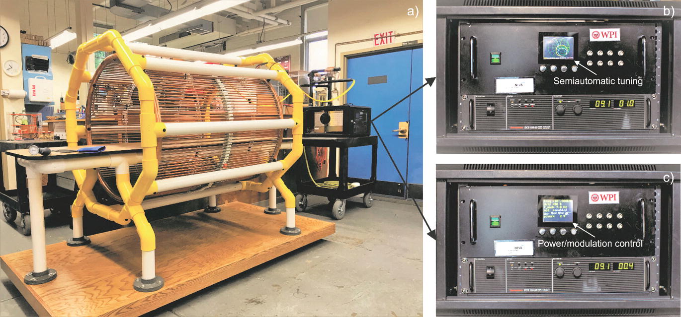
(a) Complete framed resonator coil unit with the PA. (b) Smith chart/reflection coefficient display of the power amplifier controller to be used for semiautomatic tuning for an individual subject/patient. (c) Amplifier display controlling output power and modulation frequency for harmonic modulation
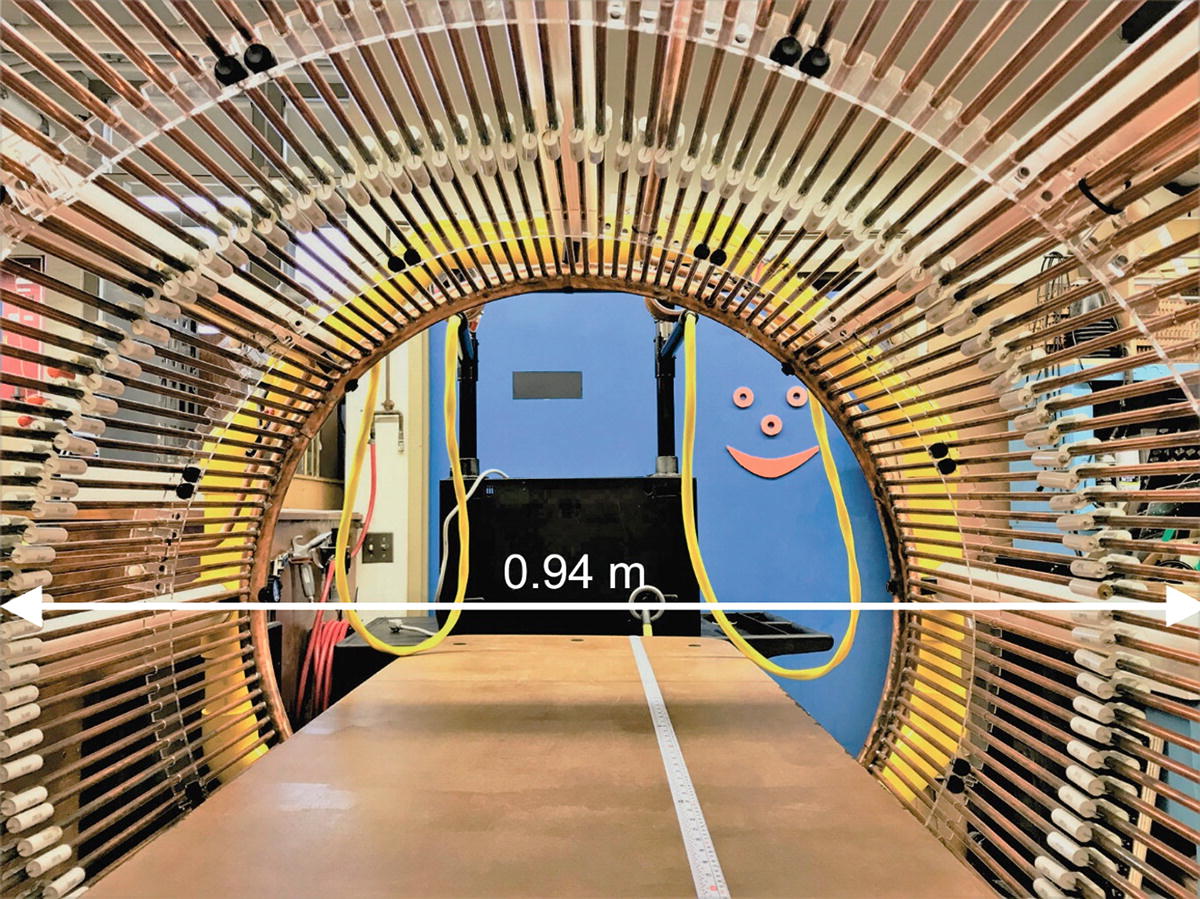
Active area of the subthreshold resonator device
This durable coil prototype was then framed, augmented with a horizontal bed, and placed horizontally to enable a subject to rest in the coil, as shown in Fig. 5.6a, which simultaneously shows the complete device setup. The entire coil frame is portable. The distance between the PA, which is connected to the inductive coupling loops of the coil via two isolated cables, can vary from 1 to 3 m, although larger distances may be possible. As mentioned above, there is no direct ohmic current path from the AC power outlet to the coil, which is an important safety feature.
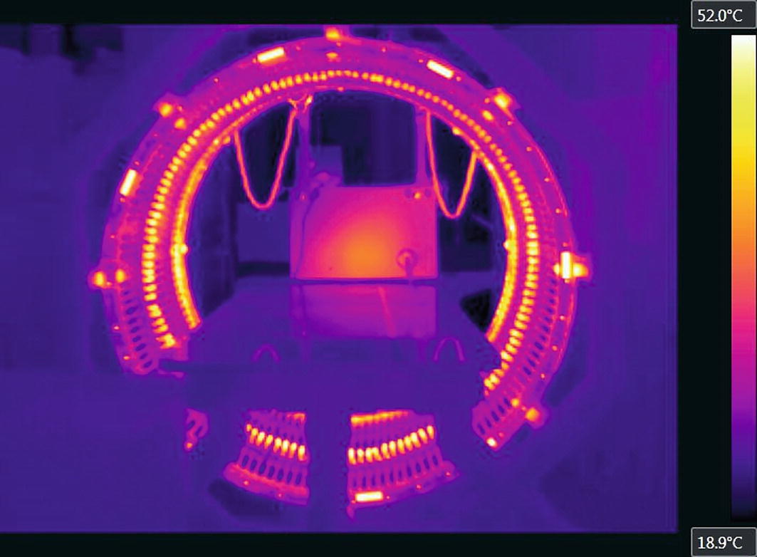
Infrared map of the coil and PA(rear) temperature distribution after 30 min of operation at maximum power obtained with FLIR A325sc IR camera
5.2.10 Quality Factor of the Resonator and the Magnetic Field Strength
The achievable field strength in the coil is determined by three factors: the strength of the PA, the quality factor Q or the “gain” of the resonator, and the coil volume. When the quality factor is high, large field values within the coil can be achieved at a modest input power.
When measured across one of its rung capacitors, the birdcage coil behaves like a parallel resonator in a narrow frequency range around the resonant mode. Using a setup with a signal generator and oscilloscope, the resonator’s quality factor has been estimated in the form:

Measured Q-factors for the coil resonator at 100 kHz and 145 kHz, respectively
Coil | f0, kHz | fL, kHz | fU, kHz | Q |
|---|---|---|---|---|
Unloaded | 145.30 | 144.567 | 145.875 | 295.8 |
Loaded | 145.28 | 144.566 | 145.879 | 292.2 |
Unloaded | 101.42 | 101.008 | 101.827 | 277.3 |
Loaded | 101.43 | 101.009 | 101.835 | 275.0 |
Characteristics of existing low-frequency RF coils given for comparison with the present resonator prototype
Ref.# | Type of the coil | Frequency, kHz | Q (unloaded) |
|---|---|---|---|
[83] | Wound birdcage coil (84 mm long and has a diameter of 73 mm) | 386 | 180 |
[84] | Wound birdcage coils and a solenoid. The diameter and the length of the coils are 70 mm | 238/425 | 100–280 |
[85] | 27 tTurn saddle coil made of Litz wire with 8 cm diameter | 373 | 105 |
[86] | 4-Coil Whiting-Lee configuration, 33 cm long | 83.6 | 100 |
[87] | Solenoidal coils; 6–46 cm in length and 4–52 cm in diameter | 210/275 | 60–30, reduced Q |
[88] | Cylindrical saddle-shaped loops (5 saddle pairs of 10 turns each), coil diameter is 26 mm | 87 | NA |
It is important to point out again that the quality factor in Table 5.1 is weakly affected by body loading, in contrast to conventional high-frequency MRI RF coils. This observation, also mentioned in Ref. [84] and other sources, is a limitation of the present electromagnetic stimulator. The RF power losses are mostly in the coil itself, and not in the human body.
B-field measurements have been performed via a calibrated single-axis coil probe located at the coil axis. The B-field magnitude was 1.01 mT at the coil center and at full power (3 kW DC) at 100 kHz. The measured and theoretical results differ by no more than 10%. At the full input power level of 3 kW, the amplitude of the resonant ring current I0 at 100 kHz in two coil rings reaches 603 A, while the amplitude of the rung current reaches 26 A.
5.3 Device Safety Estimates
5.3.1 Peripheral Nervous System (PNS) Stimulation Threshold
The present low-frequency subthreshold electrostimulation device must not exceed the PNS simulation threshold to operate safely and without unpleasant sensation. Guidelines from the International Commission on Non-Ionizing Radiation Protection (Table 5.2 of [91]) require the occupational exposure to an electric field to be limited to a value of approximately 27 V/m RMS at 100 kHz and by a value of 39 V/m RMS at 145 kHz (the so-called basic restrictions [91]). These restrictions are mainly due to limits on peripheral nerve stimulation [91] and should therefore be respected. Other relevant results on the PNS stimulation thresholds at lower frequencies are presented in Refs. [92–94].
5.3.2 Specific Absorption Rate (SAR)
Safety estimates also rely upon the levels of the specific absorption rate (SAR) within the body. The SAR is the energy absorption rate that causes body temperature to rise due to an imposed electromagnetic field. The maximum value of SAR1g in the body must be below 10 W/kg required by the FDA-accepted safety standard [95, 96]. The global-body SAR must be below the 2 W/kg limit [95, 96].
5.3.3 Method of Analysis
SAR and electric field measurements cannot be performed easily for human subjects in vivo. SAR and device performance estimates are typically derived and accepted today from computational electromagnetics (CEM) simulations performed with detailed virtual humans [97]. In this study, we use the multi-tissue CEM phantom VHP-Female v. 5.0 (female/60 year/162 cm/88 kg, obese) [97–103] derived from the cryosection dataset archived within the Visible Human Project® of the US National Library of Medicine [104]. The phantom includes about 250 individual tissues and is augmented with material property values from the IT’IS database [105]. The average-body conductivity is assigned as 0.25 S/m, which reflects a mixture of muscle and fat.
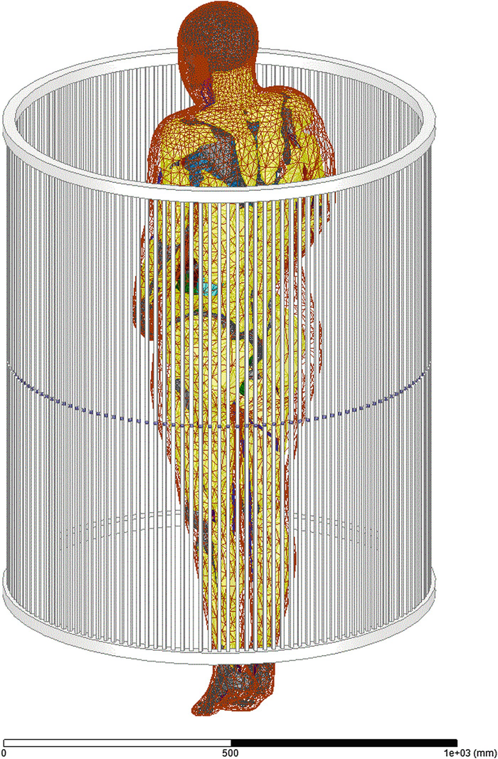
Multi-tissue CEM phantom VHP-Female v. 5.0 within the resonant coil (ANSYS 18.2.0)
Results obtained with both software packages differ by no more than 2% in the unloaded coil (field at the coil center) and by no more than 25–50% in the coil loaded with the multi-tissue human body. The latter deviation may be explained by somewhat different surface meshes.
Below we report simulations at two power levels: 1.5 kW input power and 3 kW input power. The first power level is the half power level of the amplifier driver; the second power level corresponds to full power. At full power level, the amplitude of the resonant ring current I0 in Eqs. (5.4 and 5.5) reaches 603 A, while the amplitude of the rung current reaches 26 A.
5.3.4 Electric Field Levels
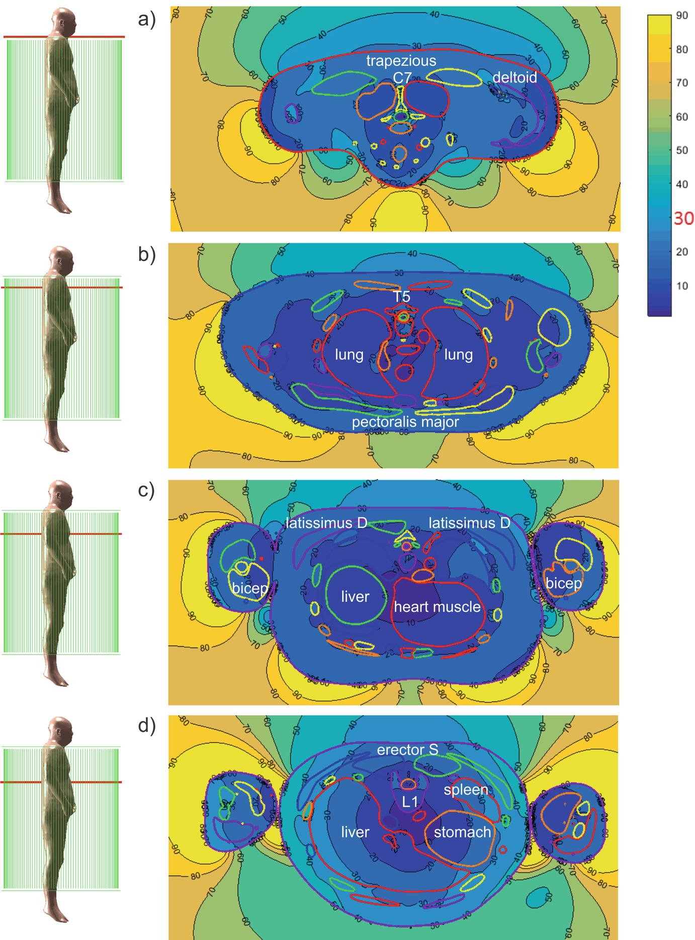
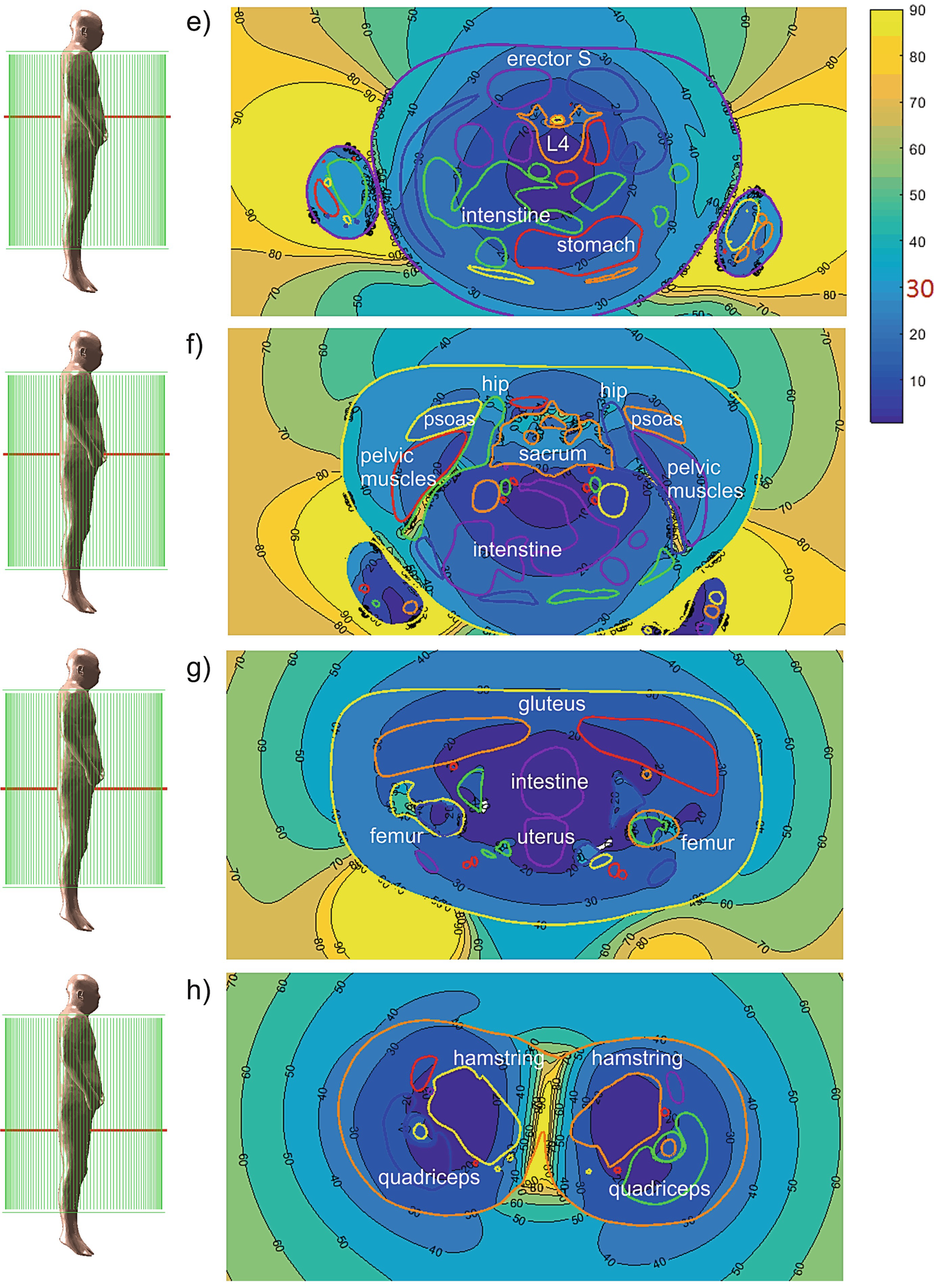
Complex RMS magnitude of the electric field (V/m) at 1500 W input power
Computed electric field levels (V/m RMS) in every individual tissue at 1.5 kW input power (ANSYS® Electromagnetic Suite 18.2.0)
Mesh | Tissue | Avg. E field (V/m RMS) | Mesh | Tissue | Avg. E field (V/m RMS) |
|---|---|---|---|---|---|
1 | Air Internal Maxillary Sinus Left | 7.7 | 39 | Cuneiform Medial right | 0.6 |
2 | Air Internal Maxillary Sinus Right | 6.9 | 40 | discC02C03 | 10.3 |
3 | Arteries | 10.5 | 41 | discC03C04 | 11.6 |
4 | Bladder | 28.0 | 42 | discC04C05 | 14.3 |
5 | C01 | 14.5 | 43 | discC05C06 | 16.9 |
6 | C02 | 13.6 | 44 | discC06C07 | 19.0 |
7 | C03 | 14.8 | 45 | discC07T01 | 20.6 |
8 | C04 | 18.5 | 46 | discL01L02 | 13.9 |
9 | C05 | 21.7 | 47 | discL02L03 | 11.5 |
10 | C06 | 26.1 | 48 | discL03L04 | 8.4 |
11 | C07 | 29.6 | 49 | discL04L05 | 4.7 |
12 | Calcaneous left | 0.6 | 50 | discL05L06 | 7.1 |
13 | Calcaneous right | 1.1 | 51 | discL06S00 | 13.8 |
14 | Cartilage1 Left | 18.5 | 52 | discT01T02 | 20.2 |
15 | Cartilage1 Right | 19.9 | 53 | discT02T03 | 17.6 |
16 | Cartilage2 Left | 19.7 | 54 | discT03T04 | 17.9 |
17 | Cartilage2 Right | 20.3 | 55 | discT04T05 | 17.4 |
18 | Cartilage3 Left | 21.2 | 56 | discT05T06 | 15.8 |
19 | Cartilage3 Right | 20.9 | 57 | discT06T07 | 15.2 |
20 | Cartilage4 Left | 22.5 | 58 | discT07T08 | 14.4 |
21 | Cartilage4 Right | 21.8 | 59 | discT08T09 | 13.6 |
22 | Cartilage5 Left | 24.3 | 60 | discT09T10 | 13.2 |
23 | Cartilage5 Right | 22.6 | 61 | discT10T11 | 12.5 |
24 | Cartilage6 Left | 36.3 | 62 | discT11T12 | 13.2 |
25 | Cartilage6 Right | 35.9 | 63 | discT12L01 | 13.4 |
26 | Cerebellum | 1.4 | 64 | Eye Left | 5.0 |
27 | Clavicle left | 55.6 | 65 | Eye Right | 5.3 |
28 | Clavicle right | 34.9 | 66 | Feet1Phalange left | 0.5 |
29 | Coccyx | 42.6 | 67 | Feet1Phalange right | 0.4 |
30 | CSF OuterShell | 3.5 | 68 | Feet2Phalange left | 0.4 |
31 | CSF Ventricles | 0.4 | 69 | Feet2Phalange right | 0.4 |
32 | Cuboid Left | 0.9 | 70 | Feet3Phalange left | 0.3 |
33 | Cuboid Right | 0.6 | 71 | Feet3Phalange right | 0.4 |
34 | Cuneiform Intermediate left | 1.3 | 72 | Feet4Phalange left | 0.4 |
35 | Cuneiform Intermediate right | 0.5 | 73 | Feet4Phalange right | 0.6 |
36 | Cuneiform Lateral left | 1.1 | 74 | Feet5Phalange left | 0.4 |
37 | Cuneiform Lateral right | 0.4 | 75 | Feet5Phalange right | 0.7 |
38 | Cuneiform Medial left | 1.3 | 76 | Femur Bone Marrow Left | 7.1 |
77 | Femur Bone Marrow Right | 8.6 | 117 | Humerus right | 23.1 |
78 | Femur left | 69.3 | 118 | Intestine | 20.6 |
79 | Femur right | 83.7 | 119 | Jaw lower | 10.0 |
80 | Fibula left | 5.9 | 120 | Kidney left | 29.3 |
81 | Fibula right | 5.4 | 121 | Kidney right | 27.2 |
82 | Gray Matter Spinal Cord | 1.5 | 122 | L01 | 27.9 |
83 | Hands1 1Phalange left | 10.2 | 123 | L02 | 25.3 |
84 | Hands1 1Phalange right | 9.5 | 124 | L03 | 22.1 |
85 | Hands1 2Phalange left | 9.5 | 125 | L04 | 19.0 |
86 | Hands1 2Phalange right | 12.1 | 126 | L05 | 14.4 |
87 | Hands1 3Phalange left | 12.2 | 127 | L06 | 17.9 |
88 | Hands1 3Phalange right | 13.4 | 128 | Liver | 29.8 |
89 | Hands2 1Phalange left | 7.6 | 129 | Lungs | 19.4 |
90 | Hands2 1Phalange right | 7.1 | 130 | Median Nerve left | 11.6 |
91 | Hands2 2Phalange left | 8.1 | 131 | Median Nerve right | 13.0 |
92 | Hands2 2Phalange right | 8.5 | 132 | Muscle Bicep left | 11.9 |
93 | Hands2 3Phalange left | 7.1 | 133 | Muscle Bicep right | 12.9 |
94 | Hands2 3Phalange right | 9.5 | 134 | Muscle Calf left | 5.0 |
95 | Hands3 1Phalange left | 6.4 | 135 | Muscle Calf right | 5.2 |
96 | Hands3 1Phalange right | 6.2 | 136 | Muscle Deltoid left | 18.7 |
97 | Hands3 2Phalange left | 8.1 | 137 | Muscle Deltoid right | 19.3 |
98 | Hands3 2Phalange right | 8.6 | 138 | Muscle Erector spinae left | 26.8 |
99 | Hands3 3Phalange left | 9.3 | 139 | Muscle Erector spinae right | 26.9 |
100 | Hands3 3Phalange right | 11.0 | 140 | Muscle Forearm Extensors left | 6.9 |
101 | Hands4 1Phalange left | 7.2 | 141 | Muscle Forearm Extensors right | 8.6 |
102 | Hands4 1Phalange right | 6.9 | 142 | Muscle Forearm Flexors left | 6.9 |
103 | Hands4 2Phalange left | 10.4 | 143 | Muscle Forearm Flexors right | 7.2 |
104 | Hands4 2Phalange right | 10.0 | 144 | Muscle Gluteus left | 27.9 |
105 | Hands4 3Phalange left | 11.1 | 145 | Muscle Gluteus right | 27.2 |
106 | Hands4 3Phalange right | 10.7 | 146 | Muscle Hamstring left | 18.9 |
107 | Hands5 1Phalange left | 9.0 | 147 | Muscle Hamstring right | 19.1 |
108 | Hands5 1Phalange right | 10.3 | 148 | Muscle Latissimus Dorsi left | 36.6 |
109 | Hands5 2Phalange left | 11.0 | 149 | Muscle Latissimus Dorsi right | 38.5 |
110 | Hands5 2Phalange right | 12.6 | 150 | Muscle Neck Combined left | 13.6 |
111 | Hands5 3Phalange left | 10.3 | 151 | Muscle Neck Combined right | 13.4 |
112 | Hands5 3Phalange right | 12.1 | 152 | Muscle Obliques left | 39.5 |
113 | Heart Muscle | 14.2 | 153 | Muscle Obliques right | 40.1 |
114 | Hip left | 60.0 | 154 | Muscle Pectoralis major left | 21.7 |
115 | Hip right | 61.4 | 155 | Muscle Pectoralis major right | 20.9 |
116 | Humerus left | 20.7 | 156 | Muscle Pectoralis minor left | 19.2 |
157 | Muscle Pectoralis minor right | 18.6 | 194 | Ribs left8 | 47.3 |
158 | Muscle Pelvic Combined left | 25.7 | 195 | Ribs left9 | 46.1 |
159 | Muscle Pelvic Combined right | 25.0 | 196 | Ribs left10 | 48.5 |
160 | Muscle Psoas left | 13.9 | 197 | Ribs left11 | 51.7 |
161 | Muscle Psoas right | 13.9 | 198 | Ribs left12 | 39.0 |
162 | Muscle Quadriceps left | 20.2 | 199 | Ribs right1 | 29.6 |
163 | Muscle Quadriceps right | 19.9 | 200 | Ribs right2 | 26.2 |
164 | Muscle Rectus Abdominis left bottom | 32.3 | 201 | Ribs right3 | 25.2 |
165 | Muscle Rectus Abdominis left middle | 34.9 | 202 | Ribs right4 | 26.1 |
166 | Muscle Rectus Abdominis left top | 39.1 | 203 | Ribs right5 | 27.2 |
167 | Muscle Rectus Abdominis right bottom | 32.5 | 204 | Ribs right6 | 29.9 |
168 | Muscle Rectus Abdominis right middle | 35.4 | 205 | Ribs right7 | 35.6 |
169 | Muscle Rectus Abdominis right top | 38.1 | 206 | Ribs right8 | 43.2 |
170 | Muscle Sartorius left | 18.6 | 207 | Ribs right9 | 53.9 |
171 | Muscle Sartorius right | 17.5 | 208 | Ribs right10 | 58.9 |
172 | Muscle Tibialis Anterior left | 6.2 | 209 | Ribs right11 | 56.9 |
173 | Muscle Tibialis Anterior right | 5.8 | 210 | Ribs right12 | 40.9 |
174 | Muscle Trapezius left | 23.6 | 211 | Sacrum | 45.7 |
175 | Muscle Trapezius right | 24.0 | 212 | Scapula left | 38.2 |
176 | Muscle Tricep left | 12.0 | 213 | Scapula right | 38.8 |
177 | Muscle Tricep right | 14.0 | 214 | Skin Shell | 27.8 |
178 | Navicular left | 1.8 | 215 | Skull | 22.8 |
179 | Navicular right | 0.7 | 216 | Sphenoid | 8.9 |
180 | Patella left | 24.3 | 217 | Spleen | 33.9 |
181 | Patella right | 22.6 | 218 | Sternum | 25.2 |
182 | Peripheral Nerve left | 17.1 | 219 | Stomach | 22.6 |
183 | Peripheral Nerve Right | 14.1 | 220 | T01 | 28.4 |
184 | Pubic Symphysis | 32.1 | 221 | T02 | 27.2 |
185 | Radial Nerve left | 14.6 | 222 | T03 | 27.2 |
186 | Radial Nerve right | 12.4 | 223 | T04 | 26.9 |
187 | Ribs left1 | 26.4 | 224 | T05 | 25.7 |
188 | Ribs left2 | 30.1 | 225 | T06 | 25.5 |
189 | Ribs left3 | 26.4 | 226 | T07 | 26.2 |
190 | Ribs left4 | 26.7 | 227 | T08 | 26.4 |
191 | Ribs left5 | 28.3 | 228 | T09 | 26.9 |
192 | Ribs left6 | 31.5 | 229 | T10 | 26.1 |
193 | Ribs left7 | 37.3 | 230 | T11 | 26.4 |
231 | T12 | 27.5 | 240 | Trabecular upper right | 0.9 |
232 | Talus left | 1.3 | 241 | Trachea Sinus | 12.4 |
233 | Talus right | 0.6 | 242 | Ulna Radius left | 8.1 |
234 | Tibia left | 8.3 | 243 | Ulna Radius right | 7.8 |
235 | Tibia right | 7.9 | 244 | Uterus | 17.3 |
236 | Tongue | 5.2 | 245 | Veins lower | 12.5 |
237 | Trabecular lower left | 0.5 | 246 | Veins upper | 12.4 |
238 | Trabecular lower right | 0.8 | 247 | White Matter | 1.0 |
239 | Trabecular upper left | 0.7 |
However, the computed local electric fields may considerably exceed the values reported in Table 5.3, in particular by 1.5–6 times. These peak values are less accurate. One potential source of the numerical error is insufficient resolution of lengthy and time-consuming full-body computations very close to the interfaces where higher fields are usually observed.
5.3.5 SAR Levels

The second critical estimate is SAR1g, which is given by averaging over a contiguous volume with the weight of 1 g,

Although this last value might appear to be relatively high, it is still within the corresponding SAR limits in MRI machines [95, 96]. In particular, the major applicable MRI safety standard, issued by the International Electrotechnical Commission (IEC) and also accepted by the U.S. Food and Drug Administration, in the normal mode (mode of operation that causes no physiological stress to patients) limits global-body SAR to 2 W/kg, global-head SAR to 3.2 W/kg, local head and torso SAR to 10 W/kg, and local extremity SAR to 20 W/kg [96]. The global SAR limits are intended to ensure a body core temperature of 39 °C or less [95, 96].
5.4 Discussion
5.4.1 Efficacy of Stimulation
The present study establishes safety and potential feasibility of the resonant neurostimulation device. However, its efficacy for treatment of chronic back pain remains largely unknown. Only clinical trials, which would ideally thoroughly investigate both short-term and cumulative effects of the suggested lower-body electromagnetic treatment, could probably answer this question. Our aim is to provide a doctor with the possibility to vary power, resonant frequency, tonic frequency, and electromagnetic pulse envelope to enable the best possible outcome during the anticipated clinical trial.
5.4.2 Integrated Effect of Stimulation
The present subthreshold stimulation device will not only affect the PNS of the lower back but also muscles, bones, tendons, and cartilage. Evidence suggests that subthreshold pulsed electromagnetic fields may stimulate osteogenesis in vitro and in vivo [106, 107], improve bone quality in osteoporotic and nonosteoporotic cell-based studies [108, 109], human studies [110–114], animal studies [115–121], and augment bone fracture healing [107, 122–124]. Further evidence suggests that TENS therapy stimulates a change in the biochemical and physiological muscle conditions that may lead to muscle relaxation [125, 126]. Some evidence also suggests that the kHz stimulation of the lower body will increase the vascular endothelial growth factor receptor on circulating hematopoietic stem cells [81], whose local niche (the bone marrow of the pelvis, femur, and sternum [127]) might be well affected by the present stimulation device.
Another extremely interesting effect of the kHz peripheral nerve stimulation observed previously in [65, 80] and implicitly in the present device is a potential for sleep improvement. It is not clear how to describe and account these integrated effects of the stimulation. We will attempt to carefully document and report prior relevant literature findings and the corresponding stimulation conditions for nerve/muscle/bone/marrow, and link them to the present stimulation conditions.
5.4.3 Operation as an EMAT
The present electrostimulation device may also operate as an electromagnetic acoustic transducer (EMAT) when a DC current is injected into the tissue via surface electrodes at a specified location. The Lorentz force will excite an ultrasonic field whose frequency is the resonant frequency.
5.4.4 Variation of Resonant Frequency
While fine tuning with a low-loss ferromagnetic load is straightforward, it is quite challenging, however, to vary the resonant frequency of a power resonator, which is usually cast in stone, allowing only a narrow tuning range. In order to do this, we have studied three different methods: a bank of electronically controlled switched power capacitors, a bank of fixed capacitors with low-resistance power relay switches, and a mechanically replaceable bolted joints-based fixed-capacitor bank. Such banks need be constructed for each of the 144 rungs of the coil in Fig. 5.6 or Fig. 5.7 in order to vary the resonant or carrier frequency over the band of, say, 10–100 kHz.
Although the first two approaches are fast and elegant, they are unfeasible. The key is the equivalent series resistance (ESR) of switched capacitors and power relay switches. Existing series switches increase ESR by about 10 times or even more. This dramatically lowers the resonator quality factor Q, resulting in about three times lower field values for a given input power. The switched capacitor solution has other serious drawbacks. Each switched capacitor block is much larger than a fixed capacitor, which will result in issues related to physically accommodating all components. On the other hand, for a relay with an exceptionally small contact resistance of 5 mΩ, Q will change by a factor of 0.6 at 100 kHz and 0.3 at 10 kHz. As the relays cycle, their contact resistance may go up significantly, especially if we do not follow the guidelines for minimum switched current (to create an arc that cleans the contacts). Thus, Q could continue dropping with cycling. Therefore, we plan to implement low-ESR mechanically replaceable bolted-joints based fixed-capacitor banks. The frequency-switching operation will take approximately 3 h.
5.5 Conclusion
In this technical study, we described a whole-body noncontact subthreshold electromagnetic stimulation device based on the concept of a familiar MRI RF resonating coil, but at a much lower resonant frequency (100–150 kHz and potentially down to 10 kHz), with a field modulation option (0.5–100 Hz), and with an input power level of up to 3 kW. Its unique features include a relatively high electric field level within the subject’s biological tissue due to the resonant effect but at low power dissipation, or SAR level, in the body itself.
We emphasize that in the low-frequency limit and at moderate field levels, SAR rather weakly correlates with the deposited electric field. One reason for this is that SAR is proportional to the field squared, and is thus quite small at moderate and low field levels. A second reason is that the tissue conductivity itself is lower (at 100 kHz, it is twice as low as at 100 MHz for muscle and five times lower for fat [105]).
Due to the large resonator volume and its noncontact nature, the subject may be conveniently located anywhere within the resonating coil over a prolonged period of time at moderate and safe electric field levels. The electric field effect does not depend on a particular body position within the resonator. The field penetration is deep everywhere in the body, including the extremities; muscles, bones, and peripheral tissues are mostly affected. Over a shorter period of time, the electric field levels could be increased to relatively large values with an amplitude of about 1 V/cm.
We envision treatment of chronic pain, and particularly neuropathic pain, as the primary potential clinical application for the device. The device enables whole-body coverage, which could be useful in the treatment of widespread pain conditions, such as painful polyneuropathy or fibromyalgia. In addition, a deeper tissue penetration can be achieved without side-effects caused by high current density in the skin associated with the traditional contact electrodes of TENS. It should be noted that these potential clinical applications are speculative and warrant empirical testing in the future.
Considerable attention has been paid to device safety including both the AC power safety and human exposure to electromagnetic fields. In the former case, we have used inductive coupling, which assures that there is no direct current path from the AC power outlet to the coil. This design enhances overall device safety at any power level, including high-power operation. As with more traditional MRI devices, no large metal objects should be located in the immediate vicinity of the coil.
Human exposure to the electromagnetic field within the coil has been evaluated by performing extensive modeling with two independent numerical methods and with an anatomically realistic multi-tissue human phantom. We have shown that the SAR levels within the body correspond to the safety standards of the International Electrotechnical Commission when the input power level of the amplifier driver does not exceed 3 kW. We have also shown that the electric field levels generally comply with the safety standards of the International Commission on Non-Ionizing Radiation Protection when the input power level of the amplifier driver does not exceed 1.5 kW.
Acknowledgments
The authors are thankful to Dr. James O’Rourke, Dr. John McNeill, Ms. Leah Morales, Mr. Brandon Weyant (all from Worcester Polytechnic Institute), MD Irina V. Zhdanova (ClockCoach), and Dr. Aapo Nummenmaa (Massachusetts General Hospital) for useful discussions. Dr. Deng is supported by the Intramural Research Program of the National Institute of Mental Health, NIH.

Open Access This chapter is licensed under the terms of the Creative Commons Attribution 4.0 International License (http://creativecommons.org/licenses/by/4.0/), which permits use, sharing, adaptation, distribution and reproduction in any medium or format, as long as you give appropriate credit to the original author(s) and the source, provide a link to the Creative Commons license and indicate if changes were made.
The images or other third party material in this chapter are included in the chapter's Creative Commons license, unless indicated otherwise in a credit line to the material. If material is not included in the chapter's Creative Commons license and your intended use is not permitted by statutory regulation or exceeds the permitted use, you will need to obtain permission directly from the copyright holder.