Identifying the propagation sources of malicious attacks in complex networks plays a critical role in limiting the damage caused by them through the timely quarantine of the sources. However, the temporal variation in the topology of the underlying networks and the ongoing dynamic processes challenge our traditional source identification techniques which are considered in static networks. In this chapter, we introduce an effective approach used in criminology to overcome the challenges. For simplicity, we use rumor source identification to present the approach.
10.1 Introduction
Rumor spreading in social networks has long been a critical threat to our society [143]. Nowadays, with the development of mobile devices and wireless techniques, the temporal characteristic of social networks (time-varying social networks) has deeply influenced the dynamic information diffusion process occurring on top of them [151]. The ubiquity and easy access of time-varying social networks not only promote the efficiency of information diffusion but also dramatically accelerate the speed of rumor spreading [91, 170].
For either forensic or defensive purposes, it has always been a significant work to identify the source of rumors in time-varying social networks [42]. However, the existing techniques for rumor source identification generally require firm connections between individuals (i.e., static networks), so that administrators can trace back along the determined connections to reach the diffusion sources. For example, many methods rely on identifying spanning trees in networks [160, 178], then the roots of the spanning trees are regarded as the rumor sources. The firm connections between users are the premise of constructing spanning trees in these methods. Some other methods detect rumor sources by measuring node centralities, such as degree, betweenness, closeness, and eigenvector centralities [146, 201]. The individual who has the maximum centrality value is considered as the rumor source. All of these centrality measures are based on static networks. Time-varying social networks, where the involved users and interactions always change, have led to great challenges to the traditional rumor source identification techniques.
In this chapter, a novel source identification method is proposed to overcome the challenges, which consists the following three steps: (1) To represent a time-varying social network, we reduce it to a sequence of static networks, each aggregating all edges and nodes present in a time-integrating window. This is the case, for instance, of rumors spreading in Bluetooth networks, for which the fine-grained temporal resolution is not available, whose spreading can be studied through different integrating windows Δt (e.g., Δt could be minutes, hours, days or even months). In each integrating window, if users did not activate the Bluetooth on their devices (i.e., offline), they would not receive or spread the rumors. If they moved out the Bluetooth coverage of their communities (i.e., physical mobility), they would not receive or spread the rumors. (2) Similar to the detective routine in criminology, a small set of suspects will be identified by adopting a reverse dissemination process to narrow down the scale of the source seeking area. The reverse dissemination process distributes copies of rumors reversely from the users whose states have been determined based on various observations upon the networks. The ones who can simultaneously receive all copies of rumors from the infected users are supposed to be the suspects of the real sources. (3) To determine the real source from the suspects, we employ a microscopic rumor spreading model to analytically estimate the probabilities of each user being in different states in each time window. Since this model allows the time-varying connections among users, it can feature the dynamics of each user. More specifically, assuming any suspect as the rumor source, we can obtain the probabilities of the observed users to be in their observed states. Then, for any suspect, we can calculate the maximum likelihood (ML) of obtaining the observation. The one who can provide the maximum ML will be considered as the real rumor source.
10.2 Time-Varying Social Networks
In this section, we introduce the primer for rumor source identification in time-varying social networks, including the features of time-varying social networks, the state transition of users when they hear a rumor, and the categorization of partial observations in time-varying social networks.
10.2.1 Time-Varying Topology
The essence of social networks lies in its time-varying nature. For example, the neighborhood of individuals moving over a geographic space evolves over time (i.e., physical mobility), and the interaction between the individuals appears and disappears in online social networks (i.e., online/offline) [151]. Time-varying social networks are defined by an ordered stream of interactions between individuals. In other words, as time progresses, the interaction structure keeps changing. Examples can be found in both face-to-face interaction networks [27], and online social networks [170]. The temporal nature of such networks has a deep influence on information spreading on top of them. Indeed, the spreading of rumors is affected by duration, sequence, and concurrency of contacts among people.
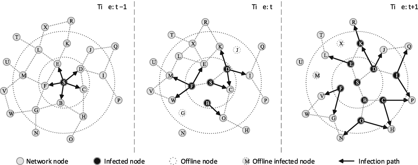
Example of a rumor spreading in a time-varying network. The random spread is located on the black node, and can travel on the links depicted as line arrows in the time windows. Dashed lines represent links that are present in the system in each time window
10.2.2 Security States of Individuals
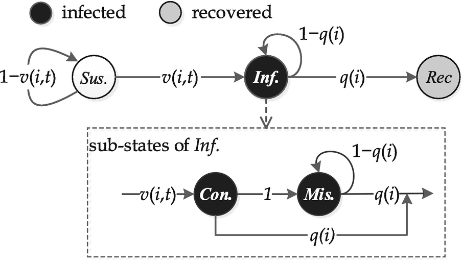
State transition of a node in rumor spreading model
To more precisely describe node states under different types of observations, we introduce two sub-states of nodes being infected: ‘contagious’ (Con.) and ‘misled’ (Mis.), see Fig. 10.2. An infected node first becomes contagious and then transit to being misled. The Con. state describes the state of nodes newly infected. More specifically, a node is Con. at time t means this node is susceptible at time t − 1 but becomes infected at time t. An misled node will stay being infected until it recovers. For instance, sensors can record the time at which they get infected, and the infection time is crucial in detecting rumor sources because it reflects the infection trend and speed of a rumor. Hence, the introduction of contagious and misled states is intrinsic to the rumor spreading framework.
10.2.3 Observations on Time-Varying Social Networks
Prior knowledge for source identification is provided by various types of partial observations upon time-varying social networks. According to previous work on static networks, we collect three categories of partial observations: wavefronts, snapshots, and sensor observations. We denote the set of observed nodes as O = {o 1, o 2, …, o n}. Following the rumor spreading in Fig. 10.1, we will explain each type of the partial observations as follows.
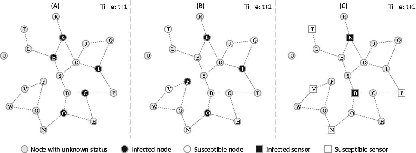
Three types of observations in regards to the rumor spreading in Fig. 10.1. (a) Wavefront; (b) Snapshot; (c) Sensor observation
Snapshot [115]: Given a rumor spreading incident, a snapshot also provides partial knowledge of the time-varying social network status. In this case, only a group of users can be observed in the latest time window when the snapshot is taken. The states of the observed users can be susceptible, infected or recovered. We use O S, O I and O R to denote the observed users who are susceptible, infected or recovered, respectively. This type of observations is the most common one in our daily life. Figure 10.3b shows an example of the snapshot in the rumor spreading in Fig. 10.1. We see that O S = {N, Q, T, V }, O I = {F, I, K, O} and O R = ∅.
Sensor Observation [146]: Sensors are a group of pre-selected users in time-varying social networks. The sensors can record the rumor spreading dynamics over them, including the security states and the time window when they get infected (more specifically, become contagious). We introduce O S and O I to denote the set of susceptible and infected sensors, respectively. For each o i ∈ O I, the infection time is denoted by t i. This type of observation is usually obtained from sensor networks. Figure 10.3c shows an example of the sensor observations in the rumor spreading in Fig. 10.1. In this case, O S = {N, P, T, V }, O I = {K, B}, and the infection time of node K is t + 1, and node B is infected at time t.
We can see that these three types of partial observations provide three different categories of partial knowledge of the time-varying social network status. Different types of observations are suitable for different circumstances in real-world applications. Readers can refer to [24, 146, 201] for further discussion on different types of partial observations. The partial knowledge together with the time-varying characteristics of social networks make the tracing back of rumor sources much more difficult.
10.3 Narrowing Down the Suspects
Current methods of source identification need to scan every node in the underlying network. This is a bottlenecks of identifying rumor sources: scalability. It is necessary to narrow down a set of suspects, especially in large-scale networks. In this section, we develop a reverse dissemination method to identify a small set of suspects. The details of the method are presented in Sect. 10.3.1, and its efficiency will be evaluated in Sect. 10.3.2.
10.3.1 Reverse Dissemination Method
In this subsection, we first present the rationale of the reverse dissemination method. Then, we show how to apply the reverse dissemination method into different types of partial observations on networks.
10.3.1.1 Rationale
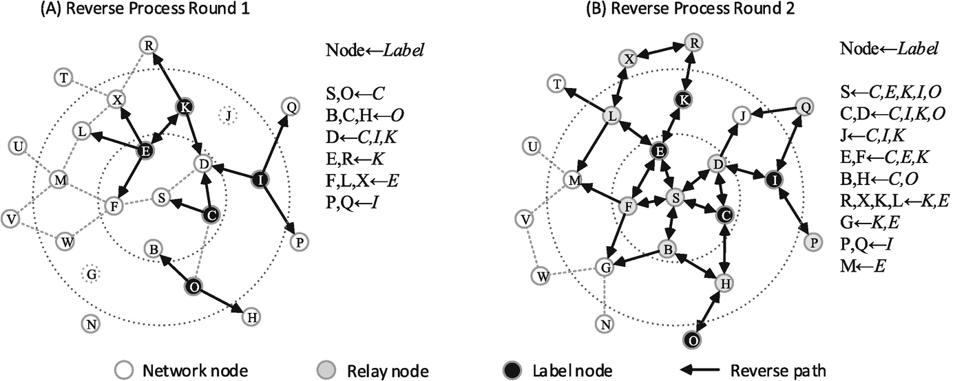
Illustration of the reverse dissemination process in regards to the wavefront observation in Fig. 10.3a. (a) The observed nodes broadcast labeled copies of rumors to their neighbors in time window t; (b) The neighbors who received labeled copies will relay them to their own neighbors in time window t − 1
We notice that the starting time for each observed node starting their reverse dissemination processes varies in different types of observations. For a wavefront, since all the observed nodes are supposed to be contagious in the latest time window, all the observed nodes need to simultaneously start their reverse dissemination processes. For a snapshot, the observed nodes stay in their states in the latest time window. Therefore, the reverse dissemination processes will also simultaneously starts from all the observed nodes. However, for a sensor observation, because the infected sensors record their infection time, the starting time of reverse dissemination for each sensor will be determined by t i. More specifically, the latest infected sensors first start their reverse dissemination processes, and then the sensors infected in the previous time window, until the very first infected sensors.
10.3.1.2 Wavefront

10.3.1.3 Snapshot

10.3.1.4 Sensor
 , where T = max{t
i|o
i ∈ O
I}. We also let the susceptible sensors o
j ∈ O
S start to reversely disseminate copies of rumors at time t=0. To match a sensor observation, it is expected a suspect u needs to satisfy the following two principles at time t. First, copies of rumors disseminated from susceptible sensors o
i ∈ O
S cannot reach node u at time t (i.e., node u is still susceptible). Second, copies of rumors disseminated from all infected sensors o
j ∈ O
I can be received by node u at time t (i.e., node u becomes contagious). Mathematically, we determine the suspects by computing their maximum likelihood, as in
, where T = max{t
i|o
i ∈ O
I}. We also let the susceptible sensors o
j ∈ O
S start to reversely disseminate copies of rumors at time t=0. To match a sensor observation, it is expected a suspect u needs to satisfy the following two principles at time t. First, copies of rumors disseminated from susceptible sensors o
i ∈ O
S cannot reach node u at time t (i.e., node u is still susceptible). Second, copies of rumors disseminated from all infected sensors o
j ∈ O
I can be received by node u at time t (i.e., node u becomes contagious). Mathematically, we determine the suspects by computing their maximum likelihood, as in 
The values of P S(u, t|o i), P C(u, t|o i), P I(u, t|o i) and P R(u, t|o i) will be calculated by the model introduced in Sect. 10.4.2. We summarize the reverse dissemination method in Algorithm 10.1.
Algorithm 10.1: Reverse dissemination
10.3.2 Performance Evaluation
We evaluate the performance of the reverse dissemination method in real time-varying social networks. Similar to Lokhov et al.’s work [108], we consider the infection probabilities and recovery probabilities to be uniformly distributed in (0,1), and the average infection and recovery probabilities are set to be 0.6 and 0.3. We also use α to denote the ratio of suspects over all nodes, α = |U|∕N, where N is the number of all nodes in a time-varying social network. The value of α ranges from 5% to 100%. We randomly choose the real source in 100 runs of each experiment. The number of 100 comes from the work in [207].
Comparison of data collected in the experiments
Dataset | MIT | Sigcom09 | ||
|---|---|---|---|---|
Device | Phone | Phone | Laptop | Laptop |
Network type | Bluetooth | Bluetooth | WiFi | WiFi |
Duration (days) | 246 | 5 | 14 | 6 |
# of devices | 97 | 76 | 143 | 45,813 |
# of contacts | 54,667 | 69,189 | 1246 | 264,004 |
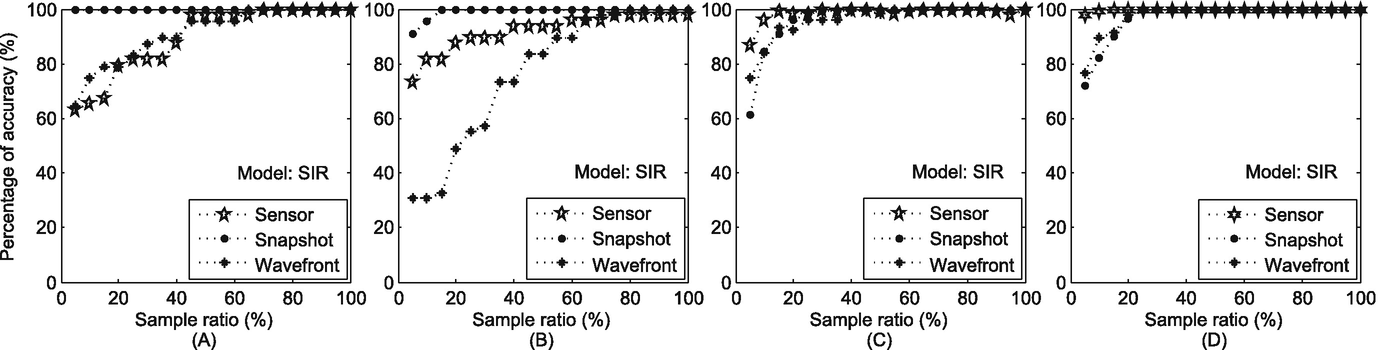
Accuracy of the reverse dissemination method in networks. (a) MIT; (b) Sigcom09; (c) Enron Email; (d) Facebook
The experiment results on real time-varying social networks show that the proposed method is efficient in narrowing down the suspects. Real-world social networks usually have a large number of users. Our proposed method addresses the scalability in source identification, and therefore is of great significance.
10.4 Determining the Real Source
Another bottleneck of identifying rumor sources is to design a good measure to specify the real source. Most of the existing methods are based on node centralities, which ignore the propagation probabilities between nodes. Some other methods consider the BFS trees instead of the original networks. These violate the rumor spreading processes. In this section, we adopt an innovative maximum-likelihood based method to identify the real source from the suspects. A novel rumor spreading model will also be introduced to model rumor spreading in time-varying social networks.
10.4.1 A Maximum-Likelihood (ML) Based Method
10.4.1.1 Rationale
 to denote the maximum likelihood of obtaining the observation when the rumor started from suspect u. Among all the suspects in U, we can estimate the real source by choosing the maximum value of the ML, as in

10.4.1.2 Wavefront
 of obtaining the wavefront O is the product of the probabilities of any observed node o
i ∈ O being contagious after time t
u. We also adopt a logarithmic function to present the computation of the maximum likelihood. Then, we have
of obtaining the wavefront O is the product of the probabilities of any observed node o
i ∈ O being contagious after time t
u. We also adopt a logarithmic function to present the computation of the maximum likelihood. Then, we have  for a wavefront, as in
10.4.1.3 Snapshot
 in a snapshot, as in
10.4.1.4 Sensor
 where
where  , and t
u is obtained from Algorithm 10.1. For suspect u ∈ U, the maximum likelihood
, and t
u is obtained from Algorithm 10.1. For suspect u ∈ U, the maximum likelihood  of obtaining the observation is the product of the probability of any sensor o
i to be in its observed state at time
of obtaining the observation is the product of the probability of any sensor o
i to be in its observed state at time  . Then, we have the logarithmic form of the calculation for
  in a sensor observation, as in
 can be calculated in the rumor spreading model in Sect. 10.4.2. We summarize the method of determining rumor sources in Algorithm 10.2.
Algorithm 10.2: Targeting the suspect
10.4.2 Propagation Model
In this subsection, we introduce an analytical model to present the spreading dynamics of rumors in time-varying social networks. The state transition of each node follows the SIR scheme introduced in Sect. 10.2.2. For rumor spreading processes among users, we use this model to calculate the probabilities of each user in various states.
![$$\displaystyle \begin{aligned} v(i,t) = 1 - \prod_{j\in N_i}[1-\eta_{ji}(t)\cdot P_I(j,t-1)], \end{aligned} $$](../images/466717_1_En_10_Chapter/466717_1_En_10_Chapter_TeX_Equ9.png)
![$$\displaystyle \begin{aligned} P_S(i,t) = [1-v(i,t)]\cdot P_S(i,t-1). \end{aligned} $$](../images/466717_1_En_10_Chapter/466717_1_En_10_Chapter_TeX_Equ10.png)


 to match the observation in time window t, given that the rumor source is the suspicious user u in Sect. 10.4.1.
10.5 Evaluation
In this section, we evaluate the efficiency of our source identification method. The experiment settings are the same as those presented in Sect. 10.3.2. Specifically, we let the sampling ratio α range from 10% to 30%, as the reverse dissemination method has already achieved a good performance with α dropping in this range.
10.5.1 Accuracy of Rumor Source Identification
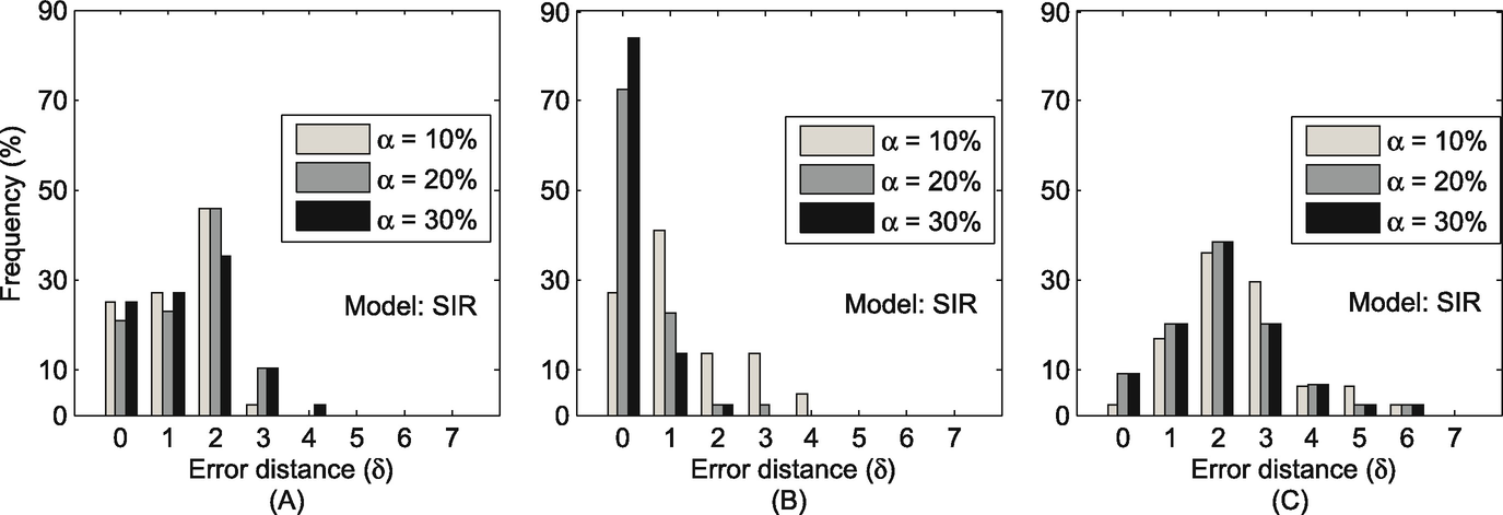
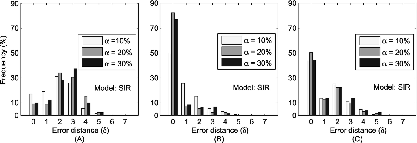
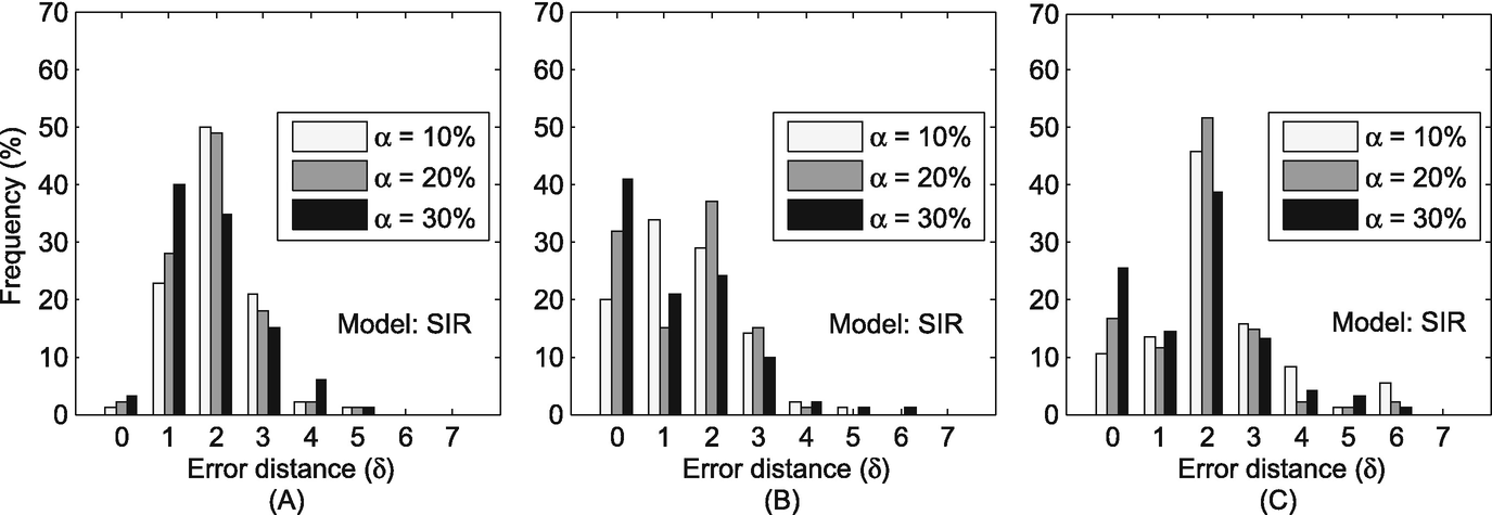
We evaluate the accuracy of our method in this subsection. We use δ to denote the error distance between a real source and an estimated source. Ideally, we have δ = 0 if our method accurately captures the real source. In practice, we expect that our method can accurately capture the real source or a user very close to the real source (i.e., δ is very small). As the user close to the real source usually has similar characteristics with the real source, quarantining or clarifying rumors at this user is also very significant to diminish the rumors [160].
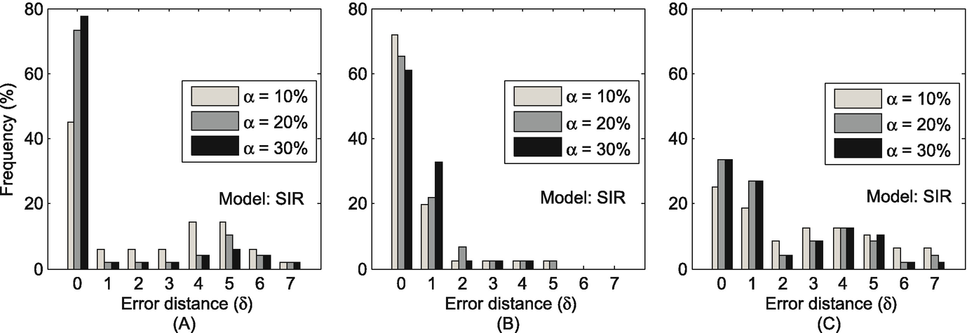
The distribution of error distance (δ) in the MIT Reality dataset. (a) Sensor; (b) Snapshot; (c) Wavefront
The distribution of error distance (δ) in the Sigcom09 dataset. (a) Sensor; (b) Snapshot; (c) Wavefront
The distribution of error distance (δ) in the Enron Email dataset. (a) Sensor; (b) Snapshot; (c) Wavefront
The distribution of error distance (δ) in the Facebook dataset. (a) Sensor; (b) Snapshot; (c) Wavefront
Compared with previous work, our proposed method is superior because our method can work in time-varying social networks rather than static networks. Our method can achieve around 80% of all experiment runs that accurately identify the real source or an individual very close to the real source. However, the previous work of [178] has theoretically proven their accuracy was at most 25% or 50% in tree-like networks, and their average error distance is 3–4 hops away.
10.5.2 Effectiveness Justification
We justify the effectiveness of our ML-based method from three aspects: the correlation between the ML of the real sources and that of the estimated sources, the accuracy of estimating rumor spreading time, and the accuracy of estimating rumor infection scale.
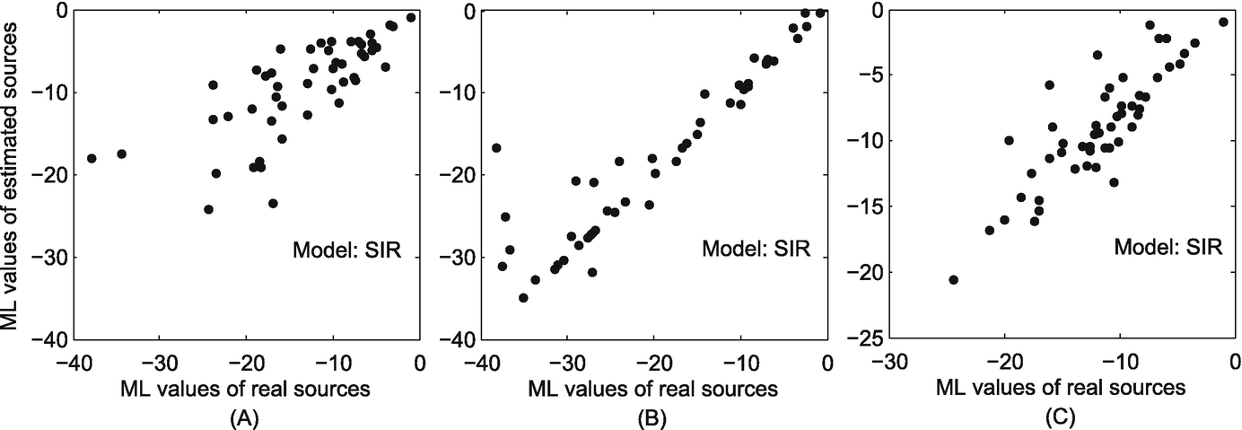
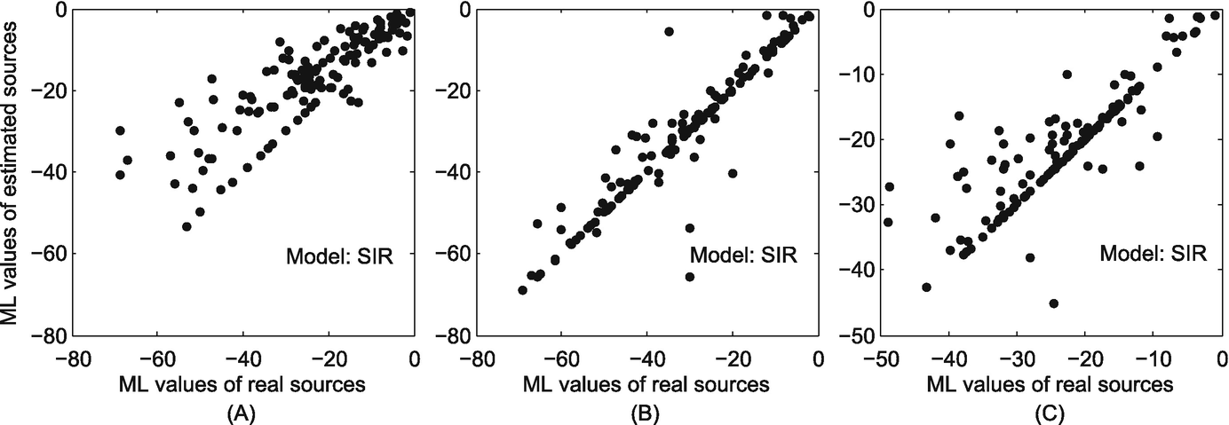
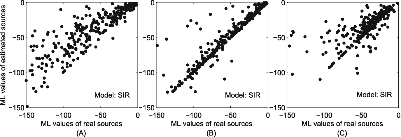
10.5.2.1 Correlation Between Real Sources and Estimated Sources
We investigate the correlation between the real sources and the estimated sources by examining the correlation between their maximum likelihood values. For different types of observation, the maximum likelihood of an estimated source can be obtained from Eqs. (10.6), (10.7) or Eq. (10.8), i.e.,  . The maximum likelihood of a real source is obtained by replacing u
∗ and t
∗ as the real source and the real rumor spreading time, respectively. If the estimated source is in fact the real source, their maximum likelihood values should present high correlation.
. The maximum likelihood of a real source is obtained by replacing u
∗ and t
∗ as the real source and the real rumor spreading time, respectively. If the estimated source is in fact the real source, their maximum likelihood values should present high correlation.
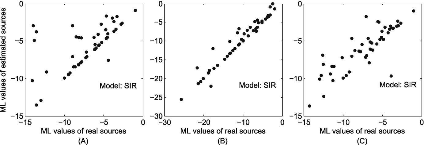
The correlation between the maximum likelihood of the real sources and that of the estimated sources in the MIT reality dataset. (a) Sensor observation; (b) Snapshot observation; (c) Wavefront observation
The correlation between the maximum likelihood of the real sources and that of the estimated sources in the Sigcom09 dataset. (a) Sensor observation; (b) Snapshot observation; (c) Wavefront observation
The correlation between the maximum likelihood of the real sources and that of the estimated sources in the Enron Email dataset. (a) Sensor observation; (b) Snapshot observation; (c) Wavefront observation
The correlation between the maximum likelihood of the real sources and that of the estimated sources in the Facebook dataset. (a) Sensor observation; (b) Snapshot observation; (c) Wavefront observation
The strong correlation between the ML values of the real sources and that of the estimated sources in time-varying social networks reflects the effectiveness of our ML-based method.
10.5.2.2 Estimation of Spreading Time
Accuracy of estimating rumor spreading time
Environment settings | Estimated spreading time | ||||
|---|---|---|---|---|---|
Observation | T | MIT | Sigcom09 | ||
Sensor | 2 | 2± 0 | 2±0 | 2±0 | 1.787±0.411 |
4 | 4.145± 0.545 | 3.936± 0.384 | 4.152± 0.503 | 3.690± 0.486 | |
6 | 6.229±0.856 | 5.978±0.488 | 6.121±0.479 | 5.720±0.604 | |
Snapshot | 2 | 1.877±0.525 | 2.200±1.212 | 2.212±0.781 | 2.170±0.761 |
4 | 3.918± 0.862 | 3.920± 0.723 | 3.893± 0.733 | 4.050± 0.716 | |
6 | 6.183±1.523 | 6.125±1.330 | 5.658±1.114 | 5.650±1.266 | |
Wavefront | 2 | 2±0 | 2±0 | 2±0 | 1.977±0.261 |
4 | 4.117± 0.686 | 4± 0 | 3.984± 0.590 | 4.072± 0.652 | |
6 | 6±0 | 5.680±1.096 | 5.907± 0.640 | 5.868±0.864 | |
As shown in Table 10.2, we analyze the means and the standard deviations of the estimated spreading time. We see that the means of the estimated spreading time are very close to the real spreading time, and most results of the standard deviations are smaller than 1. Especially when the spreading time T = 2, our ML-based method in sensor observations and wavefront observations can accurately estimate the spreading time in the MIT reality, Sigcom09 and Enron Email datasets. The results are also quite accurate in the Facebook dataset. From Table 10.2, we can see that our method can estimate the spreading time with extremely high accuracy in wavefront observations, and relatively high accuracy in snapshot observations.
Both the means and standard deviations indicate that our method can estimate the real spreading time with high accuracy. The accurate estimate of the spreading time indicates that our method is effective in rumor source identification.
10.5.2.3 Estimation of Infection Scale
We further justify the effectiveness of our ML-based method by investigating its accuracy in estimating the infection scale of rumors provided by the second byproduct in Eq. (10.5). We expect that the ML-based method can accurately estimate the infection scale of each propagation incident. Particularly, we let the rumor spreading initiate from the node with largest degree in each full time-varying social network and spread for six time windows in experiments.
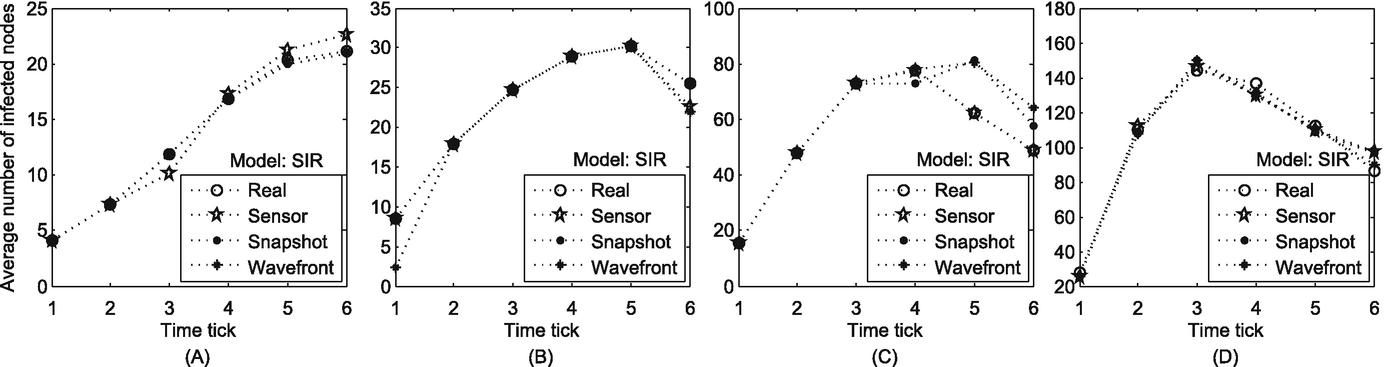
The accuracy of estimating infection scale in real networks. (a) MIT; (b) Sigcom09; (c) Enron Email; (d) Facebook
To summarize, all of the above evaluations reflect the effectiveness of our method from different aspects: the high correlation between the ML values of the real sources and that of the estimated sources, the high accuracy in estimating spreading time of rumors, and the high accuracy of the infection scale.
10.6 Summary
In this chapter, we explore the problem of rumor source identification in time-varying social networks that can be reduced to a series of static networks by introducing a time-integrating window. In order to address the challenges posted by time-varying social networks, we adopted two innovative methods. First, we utilized a novel reverse dissemination method which can sharply narrow down the scale of suspicious sources. This addresses the scalability issue in this research area and therefore dramatically promotes the efficiency of rumor source identification. Then, we introduced an analytical model for rumor spreading in time-varying social networks. Based on this model, we calculated the maximum likelihood of each suspect to determine the real source from the suspects. We conduct a series of experiments to evaluate the efficiency of our method. The experiment results indicate that our methods are efficient in identifying rumor sources in different types of real time-varying social networks.
There is some future work can be done in identifying rumor sources in time-varying networks. There are also many other models of rumor propagation, such as the models in [117, 128]. These models can be basically divided into two categories: the macroscopic models and the microscopic models. The macroscopic models, which are based on differential equations, only provide the overall infection trend of rumor propagation, such as the total number of infected nodes [207]. The microscopic models, which are based on difference equations, not only provide the overall infection status of rumor propagation, but they also can estimate the probability of an arbitrary node being in an arbitrary state [146]. In the field of identifying propagation sources, researchers generally choose microscopic models, because it requires to estimate which specific node is the first one getting infected. As far as we know, so far there is no work that is based on the macroscopic models to identify rumor sources in social networks. Future work may also investigate combining microscopic and macroscopic models, or even adopting the mesoscopic models [118, 124], to estimate both the rumour sources and the trend of the propagation. There are also many other microscopic models other than the SIR model adopted in this chapter, such as the SI, SIS, and SIRS models [146, 201]. As we discussed in Sect. 10.2.2, people generally will not believe the rumor again after they know the truth, i.e., after they get recovered, they will not transit to other states. Thus, the SIR model can reflect the state transition of people when they hear a rumor. We also evaluate the performance of the proposed method on the SI model. Since the performance of our method on the SI model is similar to that on the SIR model, we only present the results on the SIR model in this chapter.