The global diffusion of epidemics, computer viruses and rumors causes great damage to our society. One critical issue to identify the multiple diffusion sources so as to timely quarantine them. However, most methods proposed so far are unsuitable for diffusion with multiple sources because of the high computational cost and the complex spatiotemporal diffusion processes. In this chapter, we introduce an effective method to identify multiple diffusion sources, which can address three main issues in this area: (1) How many sources are there? (2)Where did the diffusion emerge? (3) When did the diffusion break out? For simplicity, we use rumor source identification to present the approach.
11.1 Introduction
With the rapid urbanization and advancements in communication technologies, the world has become more interconnected. This not only makes our daily life more convenient, but also has made us vulnerable to new types of diffusion risks. These diffusion risks arise in many different contexts. For instance, infectious diseases, such as SARS [123], H1N1 [62] or Ebola [168], have spread geographically and killed hundreds of thousands or even millions of people. Computer viruses, like Cryptolocker and Alureon, cause a good share of cyber-security incidents [119]. In the real world, rumors often emerge from multiple sources and spread incredibly fast in complex networks [62, 123, 142, 168]. After the initial outbreak of rumor diffusion, the following three issues often attract people’s attention: (1) How many sources are there? (2) Where did the diffusion emerge? and (3) When did the diffusion breakout?
In the past few years, researchers have proposed a series of methods to identify rumor diffusion sources in networks. These methods mainly focus on the identification of a single diffusion source in networks. For example, Shah and Zaman [160] proposed a rumor-center method to identify rumor sources in networks under complete observations. Essentially, they consider the rumor source as the node that has the maximum number of distinct propagation paths to all the infected nodes. Zhu and Ying [203] proposed a Jordan-center method, which utilizes a sample path based approach, to detect diffusion sources in tree networks with snapshot observations. Luo et al. [115] derived the Jordan-center method based on a different approach. Shah and Zaman [161] proved that, even in tree networks, the rumor source identification problem is a #P-complete problem, which is at least as hard as the corresponding NP problem. The problem becomes even harder for generic networks. However, due to the extreme complexity of the spatiotemporal rumor propagation process and the underlying network structure, few of existing methods are proposed for identifying multiple diffusion sources. Luo et al. [114] proposed a multi-rumor-center method to identify multiple rumor sources in tree-structured networks. The computational complexity of this method is O(n k), where n is the number of infected nodes and k is the number of sources. It is too computationally expensive to be applied in large-scale networks with multiple diffusion sources. Chen et al. [32] extended the Jordan-center method from single source detection to the identification of multiple sources in tree networks. However, the topologies of real-world networks are far more complex than trees. Fioriti et al. [58] introduced a dynamic age method to identify multiple diffusion sources in general networks. They claimed that the ‘oldest’ nodes, which were associated to those with largest eigenvalues of the adjacency matrix, were the sources of the diffusion. Similar work to this technique can be found in [148]. However, an essential prerequisite is that we need to know the number of sources in advance.
In this chapter, we introduce a novel method, K-center, to identify multiple rumor sources in general networks. In the real world, the rumor diffusion processes in networks are spatiotemporally complex because of the combined multi-scale nature and intrinsic heterogeneity of the networks. To have a clear understanding of the complex diffusion processes, we adopt a measure, effective distance, recently proposed by Brockmann and Helbing [24]. The concept of effective distance reflects the idea that a small propagation probability between neighboring nodes is effectively equivalent to a large distance between them, and vice versa. By using effective distance, the complex spatiotemporal diffusion processes can be reduced to homogeneous wave propagation patterns [24]. Moreover, the relative arrival time of diffusion arriving at a node is independent of diffusion parameters but linear with the effective distance between the source and the node of interest. For multi-source diffusion, we obtain the same linear correlation between the relative arrival time and the effective distance of any infected node. Thereby, supposing that any node can be infected very quickly, an arbitrary node is more likely to be infected by its closest source in terms of effective distance. Therefore, to identify multiple diffusion sources, we need to partition the infection graph so as to minimize the sum of effective distances between any infected node and the corresponding partition center. The final partition centers are viewed as diffusion sources.
We propose a fast method to identify multiple rumor diffusion sources. Based on this method, we can determine where the diffusion emerged. We prove that the proposed method is convergent and the computational complexity is O(mnlogα), where α = α(m, n) is the slowly growing inverse-Ackermann function, n is the number of infected nodes, and m is the number of edges connecting them.
According to the topological positions of the detected rumor sources, we derive an efficient algorithm to estimate the spreading time of the diffusion.
When the number of sources is unknown, we develop an intuitive and effective approach that can estimate the number of diffusion sources with high accuracy.
11.2 Preliminaries
In this section, we introduce preliminary knowledge used in this chapter, including the analytic epidemic model [207] and the concept of effective distance [24]. For convenience, we borrow notions from the area of epidemics to represent the states of nodes in a network [186]. A node being infected stands for a person getting infected by a disease, viruses having compromised a computer, or a user believing a rumor. Readers can derive analogous meanings for a node being susceptible or recovered.
11.2.1 The Epidemic Model
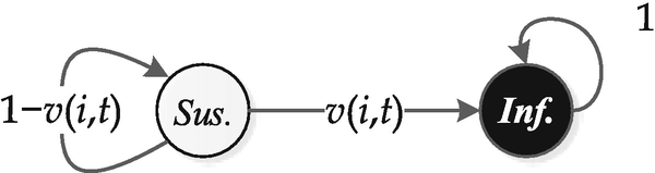
The state transition graph of a node in the SI model
![$$\displaystyle \begin{aligned} P_S(i, t) = [1 - v(i, t)] \cdot P_S(i, t - 1). \end{aligned} $$](../images/466717_1_En_11_Chapter/466717_1_En_11_Chapter_TeX_Equ1.png)

![$$\displaystyle \begin{aligned} v(i, t) = 1-\Pi_{j\in N_i} [1 - \eta_{ji}\cdot P_I(j, t - 1)], \end{aligned} $$](../images/466717_1_En_11_Chapter/466717_1_En_11_Chapter_TeX_Equ3.png)
11.2.2 The Effective Distance

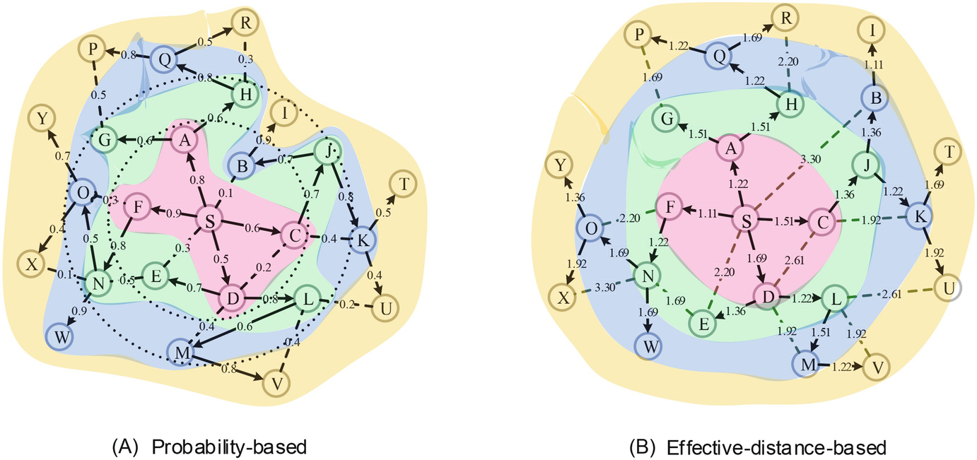
An example of altering an infection graph using effective distance. (a) An example infection graph with source S. The weight on each edge is the propagation probability. The two dot circles represent the first-order and second-order neighbors of source S. The colors indicate the infection order of nodes, e.g., nodes A, C, D and F are infected after the first time tick. Notice that the diffusion process is spatiotemporally complex. (b) The altered infection graph. The weight on each edge is the effective distance between the corresponding end nodes. Notice that the effective distances from source S to the infected nodes can accurately reflect their infection orders

From the perspective of diffusion source s, the set of shortest paths in terms of effective distance to all the other nodes constitutes a shortest path tree Ψs. Brockmann and Helbing obtain that the diffusion process initiated from node s on the original network can be represented as wave patterns on the shortest path tree Ψs. In addition, they conclude that the relative arrival time of the diffusion arriving at a node is independent of diffusion parameters and is linear with the effective distance from the source to the node of interest.
In this chapter, we will alter the original network by utilizing effective distance through converting the propagation probability on each edge to the corresponding effective distance. Then, by using the linear relationship between the relative arrival time and the effective distance of any infected node, we derive a novel method to identify multiple diffusion sources.
11.3 Problem Formulation
Before we present the problem formulation derived in this chapter, we firstly show an alternate expression of an arbitrary infection graph by using effective distance (see again Fig. 11.2). Figure 11.2a shows an example of an infection graph with diffusion source S. The colors indicate the infection order of nodes (e.g., nodes A, C, D and F were infected after the first time tick T = 1, similarly for the other nodes). Notice that the diffusion process is spatiotemporally complex, because the first-order neighbors of source S can be infected after the second time tick (e.g., node E) or even the third time tick (e.g., node B), similarly for the second-order and third-order neighbors. We then alter the infection graph by replacing the weight on each edge with the effective distance between the corresponding end nodes (see Fig. 11.2b). We notice that the effective distances from source S to all the infected nodes can accurately reflect the infection order of them. This exactly shows that the relative arrival time of an arbitrary node getting infected is linear with the effective distance between the source and the node of interest.
Suppose that at time T = 0, there are k(≥ 1) sources, S
∗ = {s
1, …, s
k}, starting the diffusion simultaneously [58, 115]. Several time ticks after the diffusion started, we got n infected nodes. These nodes form a connected infection graph G
n, and each source s
i has its infection region C
i(⊆ G
n). Let  be a partition of the infection graph such that C
i ∩ C
j = ∅. for i ≠ j. Each partition C
i is a connected subgraph in G
n and consists of the nodes whose infection can be traced back to the source node s
i. For an arbitrary infected node v
j ∈ C
i, suppose it can be infected in the shortest time, then according to our previous analysis, it will have shorter effective distance to source s
i than to any other source. Therefore, we need to divide the infection graph G
n into k partitions so that each infected node belongs to the partition with the shortest effective distance to the partition center. The final partition centers are considered as the diffusion sources.
be a partition of the infection graph such that C
i ∩ C
j = ∅. for i ≠ j. Each partition C
i is a connected subgraph in G
n and consists of the nodes whose infection can be traced back to the source node s
i. For an arbitrary infected node v
j ∈ C
i, suppose it can be infected in the shortest time, then according to our previous analysis, it will have shorter effective distance to source s
i than to any other source. Therefore, we need to divide the infection graph G
n into k partitions so that each infected node belongs to the partition with the shortest effective distance to the partition center. The final partition centers are considered as the diffusion sources.
 of the infection graph G
n. To be precise, we aim to find a partition
of the infection graph G
n. To be precise, we aim to find a partition  of G
n, to minimize the following objective function,
of G
n, to minimize the following objective function, 
Equation (11.6) is the proposed formulation for multi-source identification problem. Since, we need to find out the k centers of the diffusion from Eq. (11.6), we name the proposed method of solving the multi-source identification problem as the K-center method, which we will detail in the following section.
11.4 The K-Center Method
In this section, we propose a K-center method to identify multiple diffusion sources and the corresponding infection regions in general networks. We firstly introduce a method for network partition. Then, we derive the K-center method. Secondly, according to the estimated sources, we derive an algorithm to predict the spreading time of the diffusion. Finally, we present a heuristic algorithm to estimate the diffusion sources when the number of sources is unknown.
11.4.1 Network Partitioning with Multiple Sources

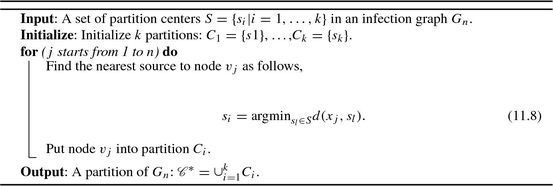
In this chapter, to satisfy Eq. (11.7), we utilize the Voronoi strategy to partition the altered infection graph obtained from Sect. 11.3. The detailed Voronoi partition process is shown in Algorithm 11.1. Future work may use community structure for network partition. Current methods for detecting community structure include strategies based on betweenness [72], information theory [152], and modularity optimization [132].
Algorithm 11.1: Network partition
11.4.2 Identifying Diffusion Sources and Regions
In this subsection, we present the K-center method to identify multiple diffusion sources. According to the objective function in Eq. (11.6), we need to find a partition  of the altered infection graph G
n, which can minimize the sum of the effective distances between each infected node and its corresponding partition center. From the previous subsection, if we randomly choose a set of sources S, Voronoi partition can split the network into subnets such that each node is associated with its nearest source. Thus, Voronoi partition can find a local optimal partition of G
n with a fixed set of sources S. However, to optimize the partition
of the altered infection graph G
n, which can minimize the sum of the effective distances between each infected node and its corresponding partition center. From the previous subsection, if we randomly choose a set of sources S, Voronoi partition can split the network into subnets such that each node is associated with its nearest source. Thus, Voronoi partition can find a local optimal partition of G
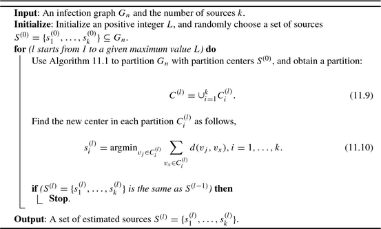
n with a fixed set of sources S. However, to optimize the partition  , we need to adjust the center of each partition so as to minimize the objective function in Eq. (11.6). In this chapter, we adjust the center of each partition by choosing a new center as the node that has the minimum sum of effective distances to all the other nodes in the partition. Therefore, we call this method as the K-center method. This is similar to the rumor-center method and the Jordan-center method that consider rumor centers or Jordan centers as the diffusion sources. As the name suggests, the K-center method is more specific to the multi-source identification. The detailed process of the K-center method is shown in Algorithm 11.2.
Algorithm 11.2: K-center to identify multiple sources
The following two theorems show the convergence of the proposed K-center method and its computational complexity.
Theorem 11.1
The objective function in Eq.(11.6) is monotonically decreasing in iterations. Therefore, the K-center method is convergent.
Proof
 are the estimated sources. We then use Algorithm 11.1 to partition the infection graph G
n as
are the estimated sources. We then use Algorithm 11.1 to partition the infection graph G
n as  . Thus, the objective function at iteration t becomes
 and obtain
  , such that


 such that each infected node v
j ∈ G
n will be associated to a nearest center
such that each infected node v
j ∈ G
n will be associated to a nearest center  , and obtain a new partition
  of G
n. Thus, the objective function at iteration t + 1 becomes
of G
n. Thus, the objective function at iteration t + 1 becomes 
 , we see that

Theorem 11.2
Given a infection graph G n with n nodes and m edges, the computational complexity of the K-center method is O(mnlogα), where α = α(m, n) is the very slowly growing inverse-Ackermann function [ 144 ].
Proof
From Algorithm 11.2, we know that the main difficulty of the K-center method stems from the calculation of the shortest paths between node pairs in the altered infection graph G n. Other computation in this algorithm can be treated as a constant. In this chapter, we adopt the Pettie-Ramachandran algorithm [144], to compute all-pairs shortest paths in G n. The computational complexity of the algorithm is O(mnlogα), where α = α(m, n) is the very slowly growing inverse-Ackermann function [144]. Therefore, we have proved the theorem.
According to Theorem 11.1, we know that the proposed K-center method is well defined. We notice that the rationale of the K-center method is similar to that of the K-means algorithm in the data-mining field. Similar to the K-means algorithm, there is no guarantee that a global minimum in the objective function will be reached. From Theorem 11.2, We see that the computational complexity of the K-center method is much less than the method in [115] with O(n k), and much less than the method in [58] with O(n 3). In addition, the proposed method can be applied in general networks, whereas the other methods mainly focus on trees. Comparatively, the proposed method is more efficient and practical in identifying multiple diffusion sources in large networks.
11.4.3 Predicting Spreading Time
 of G
n and the corresponding partition centers S
∗ by using the proposed K-center method. According to the SI model in Sect. 11.2.1, the spreading time of diffusion can be estimated by the total number of time ticks of the diffusion. Then, we can predict the spreading time based on the hops between the source and the infected nodes in each partition. For an arbitrary source s
i associated with partition C
i and an arbitrary node v
j ∈ C
i, we introduce h(s
i, v
j) to denote the minimum number of hops between s
i and v
j. Therefore, the spreading time in each partition can be estimated as in
of G
n and the corresponding partition centers S
∗ by using the proposed K-center method. According to the SI model in Sect. 11.2.1, the spreading time of diffusion can be estimated by the total number of time ticks of the diffusion. Then, we can predict the spreading time based on the hops between the source and the infected nodes in each partition. For an arbitrary source s
i associated with partition C
i and an arbitrary node v
j ∈ C
i, we introduce h(s
i, v
j) to denote the minimum number of hops between s
i and v
j. Therefore, the spreading time in each partition can be estimated as in 

11.4.4 Unknown Number of Diffusion Sources
In most practical applications, the number of diffusion sources is unknown. In this subsection, we present a heuristic algorithm that allows us to estimate the number of diffusion sources.
Algorithm 11.3: K-center identification with unknown number of sources
From Sect. 11.4.3, we know that if the number of sources k is given, we can estimate the spreading time T (k) using Eq. (11.19). To estimate the number of diffusion sources, we let k start from 1 and compute the spreading time T (1). Then, we increase the number of sources k by 1 in each iteration and compute the corresponding spreading time T (k) until we find T (k) = T (k+1), i.e., the spreading time of the diffusion stays the same when the number of sources increases from k to k + 1. That is to say when the number of sources increases from k to k + 1, they can lead to the same infection graph G n. We then choose the number of diffusion sources as k (or k + 1). The detailed process of the K-center method with unknown number of sources is shown in Algorithm 11.3. We evaluate this heuristic algorithm in Sect. 11.5.2.
To address real problems, we firstly need to get the underlying network over which the real diffusion spreads. Secondly, we need to measure the propagation probability on each edge in the network. Thirdly, according to the SI model in Sect. 11.2.1, we need to specify the length of one time tick of the diffusion properly. All of this information is crucial to source identification. However it requires big effort to obtain.
11.5 Evaluation
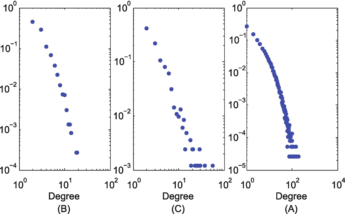
Degree distribution. (a) Power grid; (b) Yeast; (c) Facebook
Statistics of the datasets collected in experiments
Dataset | Power grid | Yeast | |
|---|---|---|---|
# nodes | 4941 | 2361 | 45,813 |
# edges | 13,188 | 13,554 | 370,532 |
Average degree | 2.67 | 5.74 | 8.09 |
Maximum degree | 19 | 64 | 223 |
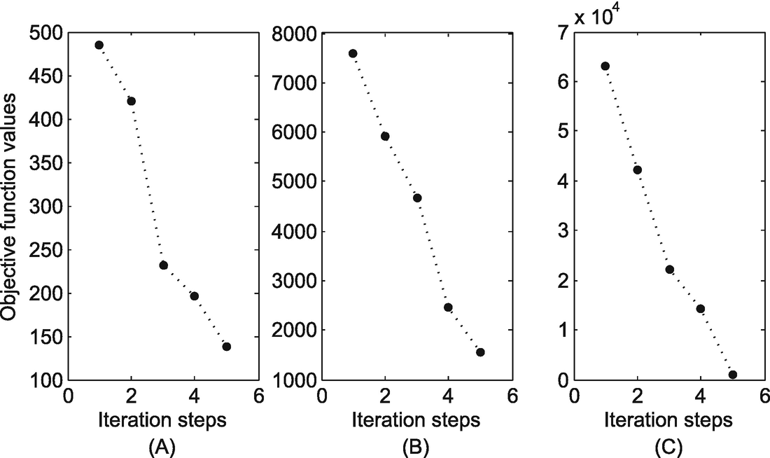
The monotonically decreasing of the objective functions. (a) Power grid; (b) Yeast; (c) Facebook
11.5.1 Accuracy of Identifying Rumor Sources
 with the real sources S
∗ = {s
1, …, s
k} so that the sum of the error distances between each estimated source and its match is minimized [160]. The average error distance is then given by
with the real sources S
∗ = {s
1, …, s
k} so that the sum of the error distances between each estimated source and its match is minimized [160]. The average error distance is then given by 
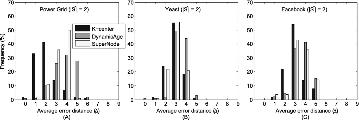
Histogram of the average error distances (Δ) in various networks when S ∗ = 2. (a) Power grid; (b) Yeast; (c) Facebook
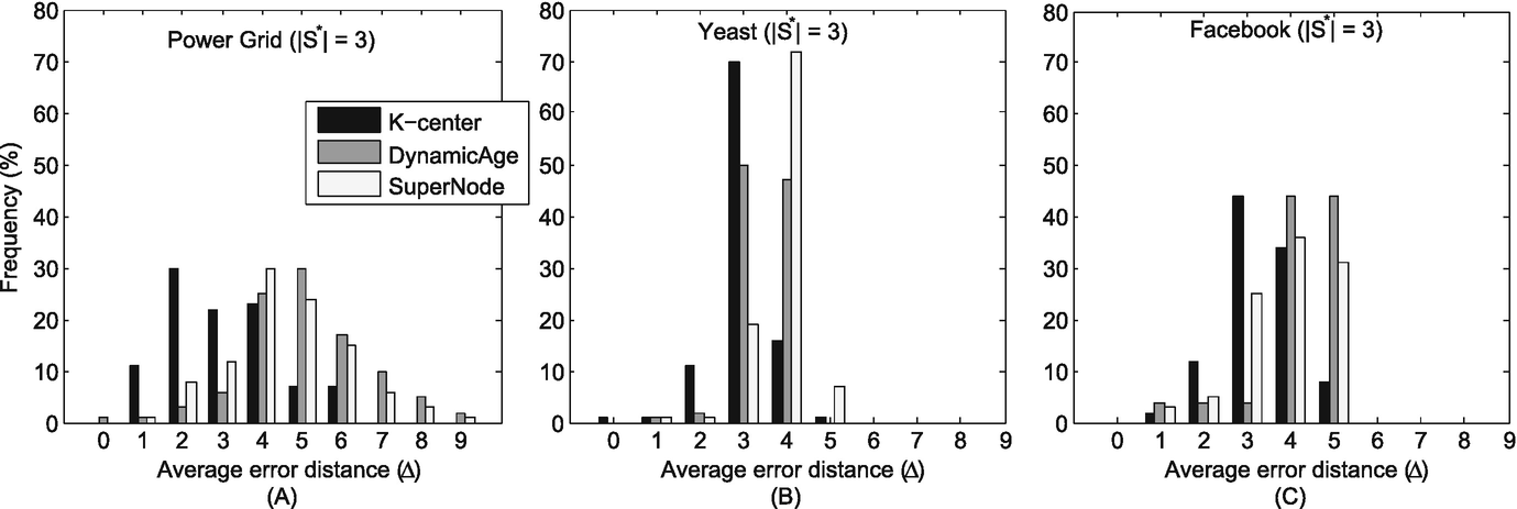
Histogram of the average error distances (Δ) in various networks when S ∗ = 3. (a) Power grid; (b) Yeast; (c) Facebook
Accuracy of multi-source identification
Experiment settings | Average error distance Δ | Infection percentage % | |||
|---|---|---|---|---|---|
Network | |S ∗| | MRC | Dynamic age | K-center | |
Power grid | 2 | 3.135 | 3.610 | 1.750 | 96.290 |
3 | 4.246 | 4.726 | 2.670 | 83.237 | |
4 | 5.331 | 6.027 | 3.240 | 78.322 | |
5 | 6.388 | 7.117 | 3.418 | 72.903 | |
Yeast | 2 | 2.700 | 3.175 | 2.680 | 89.606 |
3 | 3.520 | 3.146 | 2.733 | 74.762 | |
4 | 3.525 | 3.077 | 2.962 | 70.599 | |
5 | 3.474 | 3.050 | 2.874 | 68.563 | |
2 | 3.433 | 3.950 | 3.215 | 81.776 | |
3 | 4.667 | 4.763 | 4.073 | 76.654 | |
4 | 5.120 | 5.762 | 4.137 | 69.762 | |
5 | 5.832 | 6.701 | 4.290 | 63.723 | |
We have compared the performance of our method with two competeting methods. From the experiment results (Figs. 11.5 and 11.6, and Table 11.2), we see that our proposed method is superior to previous work. Around 80% of all experiment runs identify the nodes averagely 2–3 hops away from the real sources when there are two diffusion sources. Moreover, when there are three diffusion sources, there are also around 80% of all experiment runs identifying the nodes averagely 3 hops away from the real sources.
11.5.2 Estimation of Source Number and Spreading Time
In this subsection, we evaluate the performance of the proposed method in estimating the number of sources and predicting diffusion spreading time.
Accuracy of spreading time estimation
Experiment settings | Estimated spreading time | |||
|---|---|---|---|---|
Network | |S ∗| | T = 4 | T = 5 | T = 6 |
Power grid | 2 | 4.020 ± 0.910 | 5.050 ± 1.256 | 5.627 ± 1.212 |
3 | 4.085 ± 0.805 | 5.051 ± 0.934 | 6.006 ± 1.123 | |
Yeast | 2 | 4.600 ± 0.710 | 5.130 ± 0.469 | 5.494 ± 0.578 |
3 | 4.534 ± 0.427 | 5.050 ± 0.408 | 5.447 ± 0.396 | |
2 | 4.380 ± 1.170 | 5.246 ± 0.517 | 5.853 ± 0.645 | |
3 | 4.417 ± 0.736 | 5.378 ± 0.645 | 5.738 ± 0.467 | |
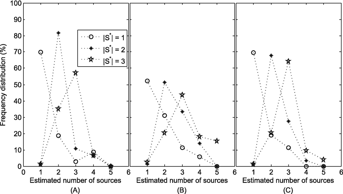
Estimate of the number of sources. (a) Yeast; (b) Power grid; (c) Facebook
The high accuracy in estimating both the spreading time and the number of diffusion sources reflects the efficiency of our method from different angles.
11.5.3 Effectiveness Justification
We justify the effectiveness of the proposed K-center method from two different aspects. Firstly, we examine the correlation between the objective function values in Eq. (11.6) of the estimated sources and those of the real sources. If they are highly correlated with each other, the objective function in Eq. (11.6) will accurately describe the multi-source identification problem. Secondly, at each time tick, we examine the average effective distances from the newly infected nodes to their corresponding diffusion sources. The linear correlation between the average effective distances and the spreading time will justify the effectiveness of using effective distance in estimating multiple diffusion sources.
11.5.3.1 Correlation Between Real Sources and Estimated Sources
We investigate the correlation between the estimated sources and the real sources by examining the correlation of their objective function values in Eq. (11.6). If the estimated sources are exactly the real sources, their objective function values f should present high correlations.
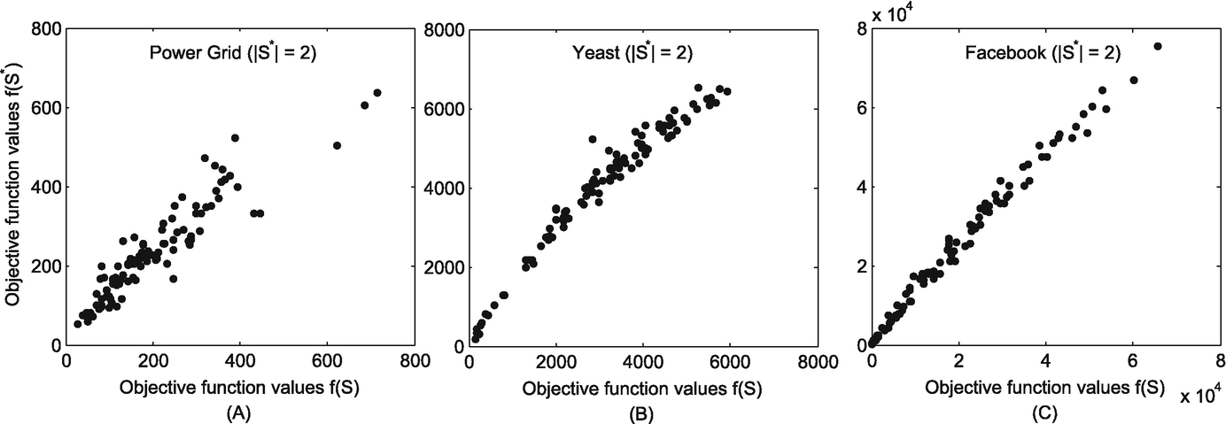
The correlation between the objective function of the estimated sources and that of the real sources when S ∗ = 2. (a) Power grid; (b) Yeast; (c) Facebook
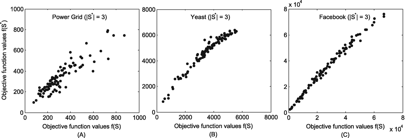
The correlation between the objective function of the estimated sources and that of the real sources when S ∗ = 3. (a) Power grid; (b) Yeast; (c) Facebook
11.5.3.2 Average Effective Distance at Each Time Tick
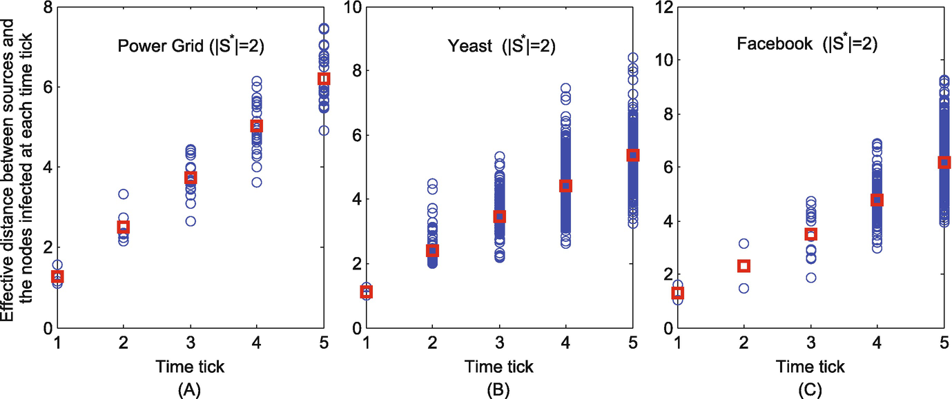
The effective distances between the nodes infected at each time tick and their corresponding sources when S ∗ = 2. (a) Power grid; (b) Yeast; (c) Facebook
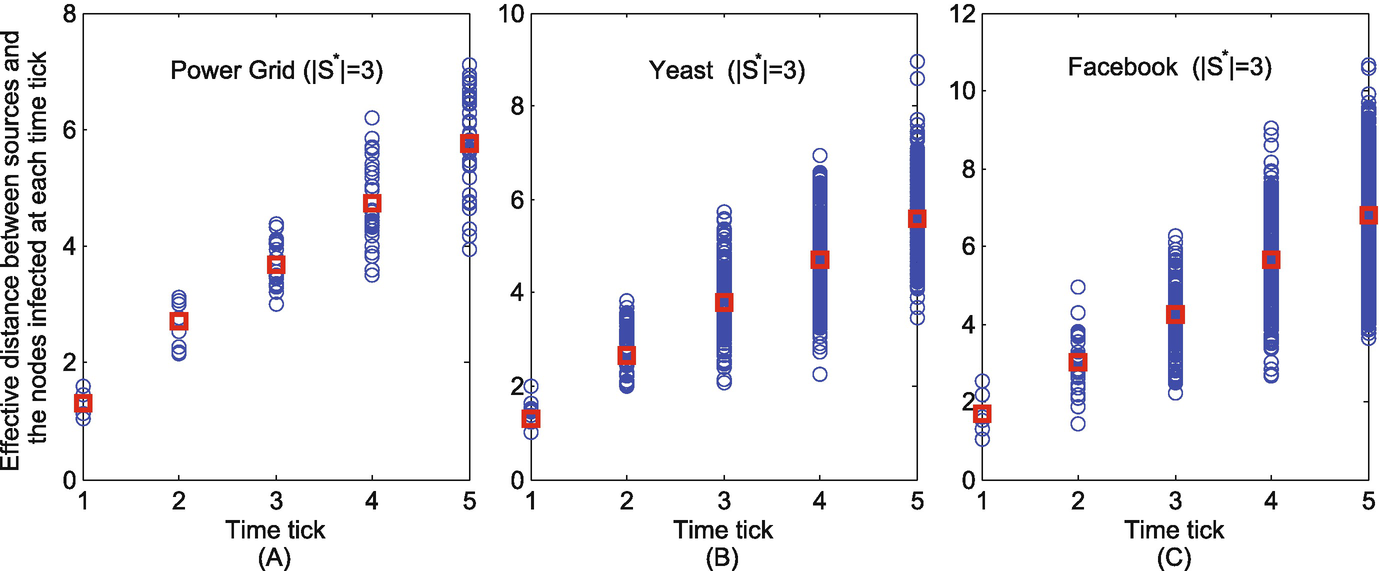
The effective distances between the nodes infected at each time tick and their corresponding sources when S ∗ = 3. (a) Power grid; (b) Yeast; (c) Facebook
As shown in Figs. 11.10 and 11.11, at each time tick, the effective distance from the nodes infected at this time tick to their corresponding sources are indicated as blue circles. Their average effective distance to the corresponding sources at each time tick is indicated as red square. It can be seen that the average effective distance is linear with the relative arrival time. This therefore justifies that the proposed K-center method is well-developed.
11.6 Summary
In this chapter, we studied the problem of identifying multiple rumor sources in complex networks. Few of current techniques can detect multiple sources in complex networks. We used effective distance to transform the original network in order to have a clear understanding of the complex diffusion pattern. Based on the altered network, we derive a succinct formulation for the problem of identifying multiple rumor sources. Then we proposed a novel method that can detect the positions of the multiple rumor sources, estimate the number of sources, and predict the spreading time of the diffusion. Experiment results in various real network topologies show the outperformance of the proposed method than other competing methods, which justify the effectiveness and efficiency of our method.
The identification of multiple rumor sources is a significant but difficult task. In this chapter, we have adopted the SI model with the knowledge of which nodes are infected and their connections. There are also some other models, such as the SIS and SIR. These models may conceal the infection history of the nodes that have been recovered. Therefore, the proposed method requiring a complete observation of network will not work in the SIS or SIR model. According to our study, we may need other techniques, e.g., the network completion, to cope with the SIS and SIR models. Future research includes the use of different models. Moreover, in the real world, we may only obtain partial observations of a network. Thus, future work includes multi-source identification with partial observations. We may also need to take community structures into account to more accurately identify multiple diffusion sources.