Preliminary of Identifying Propagation Sources

This chapter provides some primary knowledge about identifying propagation sources of malicious attacks. We first introduce different types of observations about the propagation of malicious attacks. Then, we present the maximum-likelihood estimation method adopted by many approaches in this research area. We finally introduce the evaluation metrics for source identification.

5.1 Observations on Malicious Attack Propagation

One of the major premises in propagation source identification is the observation of node states during the propagation process of malicious attacks. Diverse observations lead to a great variety of methods. According to the literature, there are three main categories of observations: complete observations, snapshots, and sensor observations. An illustration of these three categories of observations is shown in Fig. 5.1. It is clear that the snapshot and sensor observation provide much less information for identifying propagation sources compared with the complete observation.

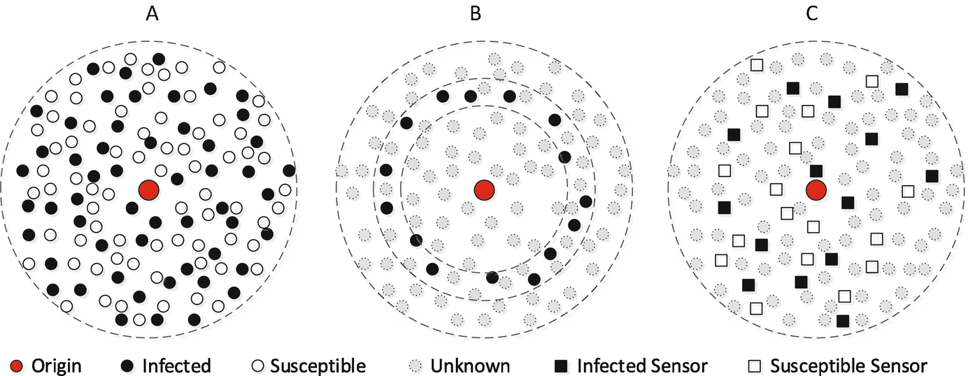
Complete Observation: Given a time t during the propagation, complete observation presents the exact state for each node in the network at time t. The state of a node stands for the node having been infected, recovered, or remaining susceptible. This type of observation provides comprehensive knowledge of a transient status of the network. Through this type of observation, source identification techniques are advised with sufficient knowledge. An example of the complete observation is shown in Fig. 5.1a.
Fig. 5.1
Illustration of three categories of observation in networks. (a) Complete observation; (b) Snapshot; (c) Sensor observation
Snapshot Observation: A snapshot provides partial knowledge of network status at a given time t. Partial knowledge is presented in four forms: (1) nodes reveal their infection status with probability μ; (2) we recognize all infected nodes, but cannot distinguish susceptible or recovered nodes; (3) only a set of nodes were observed at time t when the snapshot was taken; (4) only the nodes who were infected exactly at time t were observed. An example of the 4-th type of snapshots is shown in Fig. 5.1b.
Sensor Observation: Sensors are firstly injected into networks, and then the propagation dynamics over these sensor nodes are collected, including their states, state transition time and infection directions. In fact, sensors also stand for users or computers in networks. The difference between sensors and other nodes in networks is that they are usually monitored by network administrators in practice. Therefore, the sensors can record all details of the malicious attack propagation over them, and their life can be theoretically assumed to be everlasting during the propagation dynamics. This is different from the mobile sensor devices which may be out of work when their batteries run out. As an example, we show the sensor observation in Fig. 5.1c.

The initial methods, such as Rumor Center [160] and Dynamic Age [58], for propagation source identification require the complete observation of the network status. Later, researchers proposed source identification methods, such as Jordan Center and Concentricity based methods, for partial observations like snapshots. Researches also explored source identification methods through injecting sensors into the undering network and identifying the propagation sources based on the observations of the sensors. Accordingly, current source identification methods can be categorized into three categories in accordance with these three different types of observations, which we will introduce in the following chapters.

5.2 Maximum-Likelihood Estimation

Maximum-likelihood estimation (MLE) [37] is a method of estimating the parameters θ of a statistical model M, given the independent observed data X = {x ₁, x ₂, …, x _n}. Let us assume the probability of observing x _i in the model M given parameters θ is f(x _i|θ). Then the likelihood of having parameters θ equals to the probability of observing X given θ:

$\displaystyle \begin{aligned} \mathcal{L}(\theta|X) = f(X|\theta) = f(x_1|\theta)f(x_2|\theta)\ldots f(x_n|\theta) = \Pi{i=1}^nf(x_i|\theta). \end{aligned}$

(5.1)

$\displaystyle \begin{aligned} \mbox{log}\mathcal{L}(\theta|X) = \sum_{i=1}^n\mbox{log}f(x_i|\theta). \end{aligned}$

(5.2)

$\displaystyle \begin{aligned} \hat{\theta} = \mbox{arg max}_{\theta}~\mbox{log}~\mathcal{L}(\theta|X) = \mbox{arg max}~\sum_{i=1}^n\mbox{log}~f(x_i|\theta). \end{aligned}$

(5.3)

To find the optimal parameter $\hat {\theta }$ which best describes the observed data given the model and thus provides the largest log-likelihood value, we can solve the Eq. (5.3) or computationally search for the best solution in the parameter space. This thesis mainly adopts MLE to estimate the probability of a node being a candidate propagation source.

5.3 Efficiency Measures

Accuracy. The accuracy of a single realization is a _i = 1∕|V _top| if s ^∗∈ V _top or a _i = 0, otherwise, where s ^∗ is the true source and V _top is a group of nodes with the highest score (top scorers). The total accuracy a is an average of many realizations a _i, therefore a ∈ [0, 1]. This measure takes into account the fact that there might be more than one node with the highest score (ties are possible).
Rank. The rank is the position of the true source on the node list sorted in descending order by the score. In other words this measure shows how many nodes, according to an algorithm, is a better candidate for a source than the true source. If the real source has exactly the same score as some other node (or nodes), the true source is always below that node (these nodes) on the score list sorted in descending order. The rank takes into account the fact that an algorithm which is very poor in pointing out the source exactly (low accuracy) can be very good at pointing out a small group of nodes among which is the source.
Distance error. The distance error is the number of hops (edges) between the true source and a node designated as the source by an algorithm. If |V _top| > 1, which means that an algorithm found more than one candidate for the source, the distance error is computed as a mean shortest path distance between the real source and the top scorers.

5. Preliminary of Identifying Propagation Sources

5.1 Observations on Malicious Attack Propagation

5.2 Maximum-Likelihood Estimation

5.3 Efficiency Measures