The Children of Eve Population and Well-being in History

Chapter Three

Mortality: The Fourth Horseman

3.1 What Do People Die From?

In the developed world today, most people die from degenerative disease, the result of old age, congenital factors or life-style choices. Of the major killers, there are slight differences for men and women, and there is some variation among high-income countries to which differences in diet are a likely contributor. Historically, in contrast, death was largely associated with communicable disease, parasites, malnourishment and starvation. The same is true, to some degree, in certain less-developed countries today. The World Health Organization, for instance, estimates that 11 million infant deaths occur each year from causes that are largely preventable.¹ Absolute levels of deprivation weaken the body’s capacity to resist disease, and, although the proximate cause of death might be the communicable or parasitical diseases, the underlying cause is a lack of food and potable water, poor sanitation, lack of access to basic medical care and/or inadequate housing. Modern medicine, improved public health and hygienic practices save many individuals who otherwise would have died before these practices became widespread. The fundamental changes in the causes of death are often called the epidemiological transition and are part of the broader demographic transition.² This change and its causes and consequences are the subjects of this chapter.

Prior to modern times about one in every two children born failed to reach the age of twenty. In addition, adults tended to die earlier than they would today. There are two issues at hand. First, did the rise in individual real incomes by itself play a role in reducing the death rates, and, if so, how? Second, did the rise of scientific thinking and its promotion depend on a growth in real income (GDP adjusted for prices changes)? The evidence suggests that it did. But once started, the saving of lives could dramatically increase due to scientific breakthroughs that are more or less fortuitous or not immediately related to income. These exogenous scientific discoveries were frequently costly to implement, however. We will examine these issues later in this chapter.

With surprising frequency, in a historical context, the human population was subject to sudden, widespread disease and other deprivations. Consequently, not only was mortality high, it was highly variable. Such episodes are symbolized by the four horsemen of the apocalypse: plague (pestilence), famine, war and death. Plagues generally refer to epidemics and are diseases that rapidly spread in one area (region, nation or continent); they are called a pandemic when they occur on a worldwide scale. The virulence of each disease, the method and speed of transmission, and the susceptibility of the population all were factors in determining the death-toll of the disease. Although the spread of many diseases and their reduced effect in recent times has lessened the ravages, many of the infectious agents of diseases, called pathogens, mutate so that the medical fight against them is an on-going battle. The next horseman is famine. It is generally the result of crop or other agricultural failure brought on by unexpected changes in the weather patterns, plant disease, or an infestation of pests. A break-down of the food distribution system often compounds the problem in low income per capita countries, and it most frequently breaks down when there is a calamity such as an outbreak of plague or a war (including civil unrest). The result is malnutrition and starvation and the opportunistic diseases that thrive in the collapsed social infrastructure and the weakened bodies.³ The horsemen seldom ride alone.⁴

The causes of death today are summarized by the World Health Organization’s single cause descriptions – Table 3.1. The table distinguishes three main categories. First, worldwide, the majority of people die from non-communicable conditions, most common are: cardiovascular (heart and stroke); cancers of various types (malignant neoplasms); respiratory failure; and diseases of the digestive system. Since many of these are related to age, as humans live longer there is a greater likelihood of these conditions leading to death. The second category is communicable disease, including perinatal and nutritional conditions. Within this grouping, infectious, parasitic and respiratory disease account for over one quarter (26.0 %) of all deaths in all categories.⁵ The final category, injuries, accounts for less than 10 % of total deaths. While most of the deaths are due to agricultural and industrial accidents, domestic accidents (including transport) and misadventure, almost one-third of the total are intentional, culpable homicides and infanticides.

Table 3.1 reveals that, for any single cause of death, there is: i) a huge variation across geographic areas, and ii) a wide disparity in infant mortality. These two effects are of course linked in that communicable disease is the major killer in sub-Saharan Africa (and a large proportion of that is due to HIV/AIDS) and child mortality is very high. The variation across geographic areas is a relationship between ill health and death on one hand, and national income per capita on the other. Individual susceptibility to communicable diseases is a matter of the absolute poverty levels in the country where they live and one’s place in the income distribution. High-income citizens of low-income countries are exposed to less disease than their poorer companions. Low-income countries tend to lack the social and medical infrastructure that reduces the exposure or the spread of diseases or, once endemic, limits their consequences.

Many disease pathogens originate in domesticated animals and thus are associated with the historical rise of settled agriculture. As the numbers of domestic livestock increased, the density of the rat population also increased. Vermin are efficient carriers of pathogens. We believe certain diseases such whooping cough, scarlet fever, measles, influenza and smallpox were far less prevalent in hunter-gather societies. Some populations, such as those in the Americas prior to contact with Europe and Africa, had not acquired immunity to diseases such as smallpox because they lacked the domesticated animals found elsewhere. Table 3.2 lists some of the major communicable diseases and the domestic animals (and their companions) that carry the pathogens. Once the pathogen has made the species-leap, the disease often becomes resident in human populations. Some diseases are non-viral in origin. The parasitic disease of malaria and the bacteria that cause tuberculosis remain major killers despite attempts to eradicate them.⁶ And a further problem is the association of tuberculosis with another killer, HIV/AIDS. Since HIV/AIDS is an attack on the immune system, infected persons are less able to fight off the increasingly virulent TB.⁷ Other diseases, such as influenza, are viral. Viruses, as is well-known, mutate frequently so, for example, no influenza epidemic is exactly like the previous one.

Table 3.1 Estimates of Deaths by Causes, World and Select Areas 2002.

Source: WHO (2004), World Health Report, Geneva, Annex Table 2. http://www.who.int/whr/2004/en/09_annexes_en.pdf

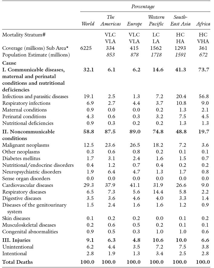
Note: WHO estimates and not those reported by specific countries.
# Mortality Stratum refers to the WHO description of death patterns in an area: VLC and VLA means “Very Low Child Mortality” and “Very Low Adult Mortality”; LC and LA means “Low Child Mortality” and “Low Adult Mortality”; HC and HA “High Child Mortality” and “High Adult Mortality”; and VHA means “Very High Adult Mortality”. For detailed definitions see the original table and WHO categories.
* refers to the population of the selected sub-area in the mortality stratum, the total population of the area is given below this number. HIV/AIDS dominates in Africa and South East Asia.

Table 3.2 Human Disease, Its Origins and Conditions of Spread.

Source: US National Library of Medicine and National Institutes of Medicine (2007), Medline Plus, Bethesda, MD: US Government. http://www.medlineplus.gov

Human Diseases	Origin	Pathogen
Measles	cattle	virus
Tuberculosis	cattle	bacterium
Smallpox	cattle (cowpox), other livestock	virus
Influenza	pigs, wild birds, domestic poultry	virus
Pertussis (Whooping Cough)	pigs and dogs	bacterium
Falciparum Malaria	chickens and ducks	parasite
West Nile Virus (flu-like with fever)	wild birds/domestic animals	virus
Bubonic plague	rodents/rat fleas	bacterium
Poor Sanitation/Overcrowding
Diarrhoea	animal fecal matter	virus, bacteria, parasites
Cholera	animal fecal matter	virus

The third category in Table 3.1 is trauma, a surprisingly large killer at 9.1 % of all deaths worldwide. While most of these deaths are accidental or a result of negligence, almost one-third is a result of intentionally delivered trauma – 2.8 of the 9.1 %. It is likely that the overall trauma-related deaths were much greater in historical periods. For instance, traumas, such as broken bones or deep cuts, can now be treated more effectively and do not lead to death. Furthermore, many of the associated effects of trauma, particularly infections, have been eliminated or reduced by modern drug therapy and hygienic practice. There is no reasonable way of knowing whether intentional trauma deaths have increased proportionately over our long history. What is known is that deadly conflict has always been with us.

Evidence for pre-Columbian North America, for instance, suggests that there was a relatively high level of violent deaths among the various population groups and that the frequency of this increased as populations became more densely settled on the land.⁸ For more modern times, since the end of the Napoleonic Wars in 1815, the approximate number of military deaths in international and civil wars (to 1980) is estimated to be about 40 million – see Table 3.3. This includes members of the military who died of infections as well as trauma, but it does not include all the private citizens who died as a result of war. Probably the greatest war-related loss of life prior to the 20th century was that during the Taiping Rebellion in China (1850–1865) with a total of military and civilian losses of 20 to 30 million. In more recent history, the Second World War had many intentional deaths that were not directly battlefield losses: the approximately 6 million victims of the Holocaust in Europe. The fire-bombing of cities added many more. But there were also deaths that were unintentional by-products of war, the results of displacement, scarcity of foodstuffs and hunger, and the spread of diseases among a weakened population, both military and civilian. The USSR suffered staggering losses in the Second World War (The Great Patriotic War from 1941 to 1945 as it was known) of approximately 17.9 million civilian deaths.⁹ Total war losses of 26.6 million were no less than 13.5 % of the 1941 population.

Table 3.3 Battle Connected Deaths in International Wars and Civil Wars, 1816–1980.

Source: Singer and Small (1982), Tables 7.3 and 16.1 and 70–1.

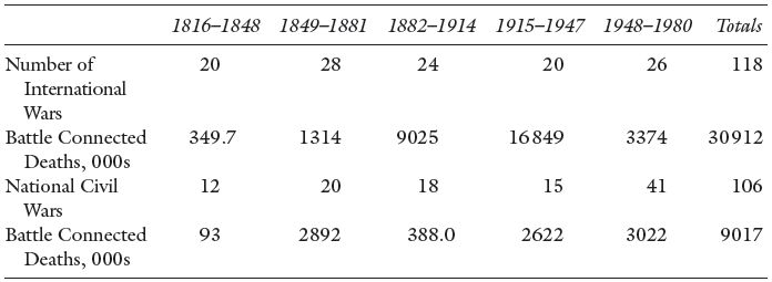
Notes : Battle connected deaths are assigned to the year in which the war began. These deaths are military and include: 1) deaths; 2) wounded who subsequently died as a result of the war; 3) deaths while in the military; and 4) in the case of civil wars, to account for guerrilla warfare, civilian casualties.

Direct military deaths in wars are generally made up of younger age males. This concentration of the deaths in one cohort, if substantial in number, has an effect on the way populations grow because of the lack of marriageable males. Thus, a cohort of women found it more difficult to find a partner as the gender ratio declined for that age group. The net consequence was a dramatic fall in the pattern of births. The slow growth of the French population in the aftermath of the Napoleonic Wars is due, in part, to this effect.

The gender or sex ratio is the number of males per 100 females – or the other way around, so check definitions carefully. It is often expressed for a cohort as, for example, the ratio of males in the age range 20–39 to the number of females in the same age range.

3.2 Infant and Child Mortality

The crude death rate (CDR) measures the number of deaths per year per 1000 individuals.¹⁰ There are many factors that influence its value so we standardize by characteristic in order to tell where the variation in the overall CDR is found. For example, the CDR is extremely sensitive to the age structure of the population. If a population has more people in the age range of greatest risk to die, the CDR will be higher. Today, for instance, we have an aging population in most countries of the world so we should expect, other things being equal, the CDR to rise since everyone drops off the peg at some point. In order to normalize for this effect demographers often calculate the number of deaths per 1000 individuals in an age range; for example, the death rate of young adults is the number of deaths in the age range 19–24 as a proportion of the population of the same age expressed per 1000. (If 2 300 people out of a population of 1 000 000 dies, the death rate is 2.3 per 1000). We know that gender is important as women are exposed to a risk that men are not: the possibility of death in childbirth. So we may wish to separate the death rate of young adults by gender. Our ability to calculate and use specific death rates is limited only by the information available.

By far, childhood represents the age of greatest historical risk of unexpected death. These death rates are traditionally broken into four parts:

neonatal mortality: deaths in the first 27 days of life;
infant mortality: deaths in the first 12 months of life;
child mortality: deaths in the first five years of life; and
youth mortality: deaths in the first 19 years of life.¹¹

Infant mortality includes neonatal deaths and the other categories are likewise inclusive. Figure 3.1 shows child mortality. But often researchers have a particular research aim for which more precision is needed, and they report the rates net of the others. For instance, Ó Gráda in his study of child death in Victorian Dublin and Belfast uses the child mortality rate where child is defined as the range of one to four years of age.¹² Each age category is chosen to highlight a particular susceptibility. To complicate matters, the clinical causes of death in history are often hard to identify because they were not known at the time. Furthermore, the symptoms were not accurately diagnosed and recorded well. So, even with modern knowledge, it is often difficult to identify the causes of death in retrospect. Even the specific age at death is often not available in historical records.

Currently, 90 % of all child deaths, those to age five, are accounted for in 43 less-developed countries. Approximately 40 % of those are actually neonatal deaths.¹³ Throughout the world the child mortality rate has fallen in recent years although the proportionate saving of life occurs least in the high mortality countries. This is often referred to as the “Matthew Effect.”¹⁴ The term expresses the tendency for the greatest benefits go to those that have the most. While this is neither wholly true nor, if true, universally true, as an inspection of recent growth rates of national incomes reveal, there is a strong historical basis for it: where you start matters! For the low-income countries these figures indicate poor living conditions, the poor health of the mothers and the general malnourishment of the population. The question is: were these the conditions of history? The answer is, alas, not straightforward.

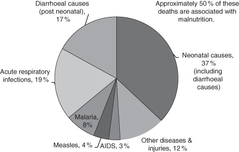
Figure 3.1 Causes of Child (Under Five) Mortality World-Wide, 2000–2003.

Source: United Nations (2004) Millennium Indicators Database.

Age-specific death rate (deaths by age): number of persons in an age bracket who die in a year, expressed as a number per 1000 in the age bracket (at the beginning of the year)

Other specific death rates: by gender; by marital status; by location; by income and … so on.

Infant mortality rate: number of children (0 to 12 months) who die in a year, expressed as a number per 1000 of children born in the year of the same age range. Also neonatal (0–28 days), child (0–4 years) and youth mortality (6–19 years) rates. (We defined these as rates above.)

Where the time span of the group is greater than one year, it is an average. Demographers use both inclusive and exclusive rates. That is, child mortality is sometimes given net of infant mortality.

First, most of the evidence for mortality rates for years before the middle of the 19th century comes from partial evidence of the death records and usually involves backward projections.¹⁵ Few jurisdictions kept or required a universal registration of deaths prior to this time. Researchers have spent much effort, and used considerable ingenuity, to amass indirect evidence that takes us back to the 16th century. Earlier than this date the historical record is written from fragmentary evidence. Nonetheless, it is consistent with the general pattern of high mortality with much geographic variation. For instance, the historical infant mortality rates were probably in the range of 200 to 250 per 1000 live births for late Tudor England and Wales.¹⁶ Similar rates have been reported for other countries including 17th century colonial US, New France, the Low Countries, France and parts of northern and western Europe. Indeed, from the mid-16th to the late 18th century there was little change in the average although there were substantial year to year variations associated the outbreaks of contagious disease, local fluctuations in agricultural productivity (income), and long-term economic swings. The rise in the late 17th century was followed by a decline to trend. The late 17th century records also suggest a difference in infant and child mortality between rural (lower) and urban (higher) mortality – farming and industrial based, respectively. Thus the infant and child mortality rates were very sensitive to the structure of the economy and how it was changing.¹⁷ A downward drift of the infant mortality rate is evident by the about the time that the gains from the industrial revolution in the late 18th century, however slight, began to have an effect on household consumption patterns. But, even in those circumstances the (mean) infant mortality remained above 150 per 1000, and it stayed there until the beginning of the 20th century.¹⁸

An alternative hypothesis is associated with Gunnar Fridlizus and Alfred Perrenoud. Drawn from their separate investigations of 17th and 18th century European countries, they claim that the declining mortality among the young was not so much a product of growing per capita income as a change in many disease patterns. This virulence theory proposes that this particular historical period witnessed a decline in the potency of certain diseases which limited their spread, albeit for unknown epidemiological reasons. Also, for the countries investigated, they claim there was neither evidence of increases in agricultural output nor broad evidence of an improved standard of living.

Even in high-income countries, the neonatal and infant death rates remained high by modern standards until very recently, although not as high as its historic heights. For example, on a world scale, infant mortality in the last 30 years rate fell to one-third of its 1971 level. Again the evidence is widespread and the rapid decline began much earlier for the high-income countries. Here shown in Figure 3.2 is the decade-by-decade decline of infant mortality since the mid-19th century for the US. For the most advanced of western European and North American countries, the infant mortality began a long downward drift some time in the early 1700s. Although varying by country, by the late 19th century infant mortality had declined to a number of approximately 150 deaths per 1000 live births (as noted above). Quantitatively, by far the most significant savings of young lives began in the very late 19th century, similar to what happened in the US.¹⁹ The precipitous fall of infant mortality rates resulted from a combination of social spending on water and sewage systems, improvement of the housing stock, and medical and hygiene practices, an important component of which were the new antiseptic procedures. We also cannot rule out the supposed decrease of the virulence of some disease pathogens. The first half of the 20th century witnessed this continued and dramatic decline that was widespread in the high income/industrialized countries and of approximately the same dimensions and timing.

Figure 3.2 Infant Mortality Rate, United States, 1850–2000 – deaths of infants 0 to 5 years old per 1000 of live births.

Source: Haines (2006) US Historical Statistics, Series Ab 920.

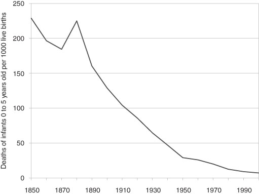
Note: Interpolated Census data.

3.3 The Probability of Death and Life Expectancy

If mortality rates are known by age of death, either from populations or samples, then life expectancy can be calculated. However, in order to know the probability of dying at any particular age, we need a large amount of historical information about a population. Only a few countries’ populations have death records that are sufficiently complete to permit gazing into the past earlier than the mid-19th century with large data samples: Canada (specifically Quebec), France, Norway, Sweden and Switzerland (Geneva) – and from which life tables are constructed.²⁰ For others we rely on relatively small samples and backward projections based on these samples. For instance, we rely for much pre-1850 data for the US on the colony/state of Massachusetts.

Gravestone, 1742
Typical gravestone from the 18th Century with its images of death: skull, cross-bones, hour-glass, spades and funeral drapes.

Source: The authors’ photograph, Cramond Kirk, 2010.

Robert Bourbeau, Jacques Légaré, and Valérie Émond have calculated the probability of death for male and female members of selected birth cohorts from 1801 to 1941 in Canada. Some of their results are in Figure 3.3.²¹ They are remarkably revealing:

Each successive birth cohort (separated by 30 or 20 years) has a lower probability of death at every age.
The probability of dying while very young (as expected) was very high but then declined rapidly by age so that, for the 1941 cohort, youths of 10 to 13 years of age were the least likely to die of any age group.
The decline in infant mortality is clearly evident by the inward shift (lower age) and steeper fall of the probability of death curves.
For both males and females there was a sharply increased risk of dying in the age range of 20 to 30 years of age except in the female 1941 birth cohort.
The pattern and level of the probability of death was roughly the same for males and females with the two exceptions: i) that noted immediately above and ii) at older ages where females generally live longer.

Figure 3.3 Probability of Dying for Selected Birth Cohorts, Canada, 1801–1940.

Source: from data in Bourbeau, Légaré, and Émond (1997).

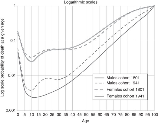
Notes: Data for the years prior to 1851 are from the Province of Quebec.

Females were exposed to the probability of death associated with giving birth – usually from an infection contracted and carried by the care-giver assisting the birth. However, as if not to be outdone, males were exposed to a different risk, that of death due to accidents, other trauma and misadventure. So the profile of mortality looked remarkably similar but for different reasons. So why are the probabilities so different for the 1941 birth cohort? Just as neonatal mortality was plummeting in the first five decades of the 20th century so was the risk of maternal death. For the 1941 birth cohort of females the risk of death due to giving birth becomes barely measurable – see later in this chapter. For the males, however, while the risk of death due to work-related accidents falls there is a new risk, death due to motor vehicle accidents, a product of affluence. This is widely supported in the North American data. Suicide rates also increased (and, for certain US inner-city youths, so did death due to gunshots).

How long did people live, on average, in early societies? The evidence is abundant but fragmentary. However, archaeological evidence from gravesites suggests that about 5000 years ago North American Indian hunter-agriculturalists had a life expectancy at birth of only about 18.9 years. In ancient Egypt (and Nubia) around 1050 BC, in an economy dominated by sedentary agriculture, life expectancy at birth was about 19.2 years. Two populations widely separated in time, geography and the economic basis for society share a common expectation of life even although the patterns of disease were different. Perhaps this defines the minimum average life expectancy in any sustainable population?²² There is considerable scholarly debate about the appropriate calculated life expectancy at birth of ancient Mediterranean peoples. It centers on the sufficiency and reliability of data and the models used for the backward projections. Some of the suggestions are: 23.0 years for Greeks of 670 BC, 26.5 for Egyptians of the Ptolemaic period and about 25.0 to 30.0 years for the Romans of the 1st century.²³ Yet, almost 1500 years later, at the beginning of the modern era, and using better evidence, the life expectancy at birth was in the same range, only 23.6 for the Swiss in Geneva (1625 to 1649).²⁴

If we judge by the later Geneva data, there was an increase in life expectancy over the course of the 17th century which is consistent with modest growth in agricultural productivity. For Europe in general, as noted earlier, the rise of life expectancy in the 17th and 18th centuries has been attributed to the deceased virulence of some diseases, the virtual disappearance of bubonic plague, and the first treatment to counteract smallpox (still relatively primitive). All undoubtedly were contributors. But by the 1700s it was Northern Europe which led the mortality decline. But why was Northern Europe so different? In Sweden, for instance, life expectancy at birth was 38.3 for females (lower for males) in the 1750s. This was approximately five full years greater than for similar countries in North Western Europe. France at this time had a life expectancy of 28.7 years.²⁵ Several explanations account for Sweden’s lead in lowering the probability of death. First was the early appearance of public health awareness under enlightened government policies. For instance, Sweden introduced training for midwives about this time, well in advance of other European countries. Second, was the rise in per capita income in the urban areas, which was probably greater than that in comparable areas of England and Wales. Third, there was a lower incidence of infant mortality from exposure to water-borne bacterial disease both because i) there was increased understanding of the association between poor public hygiene and disease, and ii) the promotion of breast-feeding which reduces the hazard of exposing young children to bacteria-infected water.²⁶ No one explanation of the falling mortality likely dominates in the first phases of the great mortality decline; all had a role. Unfortunately, we lack the detailed side-by-side information for most countries but it does seem that the Nordic countries led the (albeit slow) decline in mortality in the 18th century.²⁷

With the fall of mortality rates in North America and Western Europe, life expectancies at birth rose. Of course, one of the arithmetic reasons for the great decline, especially evident in the late 19th and early 20th centuries, was decline in the percentage of the population at greatest risk, the young. As explored in the next chapter, the decline in fertility also played a role so we cannot assume simple cause and effect. As historians, probably the most frequently neglected question and the one most relevant to ask is: was the change in the rate (death, fertility, disease, etc.) brought about by a change in the age-structure of the population?

Cohort Analysis

Cohort: the population (or a sample) born in a certain time period or a group fixed in time by some shared characteristic, e.g.: all females born in Scotland in the years 1871–1876; and all members of the 1963 graduating class of Princeton University.

In Figure 3.4, the life expectancy histories, for males, for several countries whose death rates have today reached very low levels are reported. Following this (in Figure 3.5) are (separate) male and female life expectancies for the United States in the 20th century. That is, the time series of life expectancy at birth (and the corresponding fall in the age specific death rates) broadly follows the rapid rise in the Western European and North American economies (measured in real GDP growth) in the late 19th and 20th centuries. Naturally, the death rates and corresponding life expectancies have stabilized in recent years. We may anticipate that any further changes will be relatively modest. Thus, for the developed western economies and some Asian ones the historical mortality pattern conforms to that predicted by the demographic transition. Of course, there were variations both over time and between countries which will be explored later. The current low income countries have life expectancies at birth that are much higher than those of, for example, Western Europe of the early 17th century. Sub-Saharan life expectancies today are roughly comparable to those of North America and Western Europe of 150 years ago.

Figure 3.4 Life Expectancy at Birth for Males, Canada, Sweden, United Kingdom and United States, 1750–2000.

Source: Bourbeau, Légaré, and Émond (1997); Haines (2006), Human Mortality Database (current): Haines (2006), US Historical Statistics, AB 644; Office of Health Economics, UK (current): Smith and Bradshaw (2006); Statistics Canada, Catalogue no. 91F0015MPE, Table 4.1.

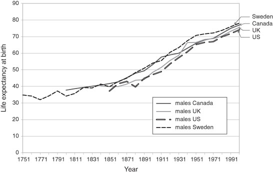
Note: The data are for either the year noted or the census one year earlier. Canadian data up to 1921 are based on ten-year cohort data and subsequently on three-year averages. The 20th century US data are the recalculation of Smith and Bradshaw.

Figure 3.5 Life Expectancy at Birth of US Males and Females in the 20th Century.

Source: data from Smith and Bradshaw (2006).

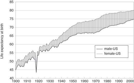
Note: The great dip in the life expectancies of both genders is a result of the influenza epidemic of 1919 – see Chapter Ten.

A pioneering study of life expectancies in the United States was conducted by the 18th century Harvard professor, Edward Wigglesworth. He estimated the life expectancy at birth (for both sexes combined) at 36.4 years at the end of the American Revolution (1789).²⁸ Life expectancy at age 20 in 1789 was 34.2 years, which is slightly lower than that of Geneva citizens for the same decade, the 1780s. Thanks to the current research of the scholar Michael Haines, we now have detailed life tables for the US from 1850 onward – some of these data are in Figure 3.5. From 1850 to 1900 there was a gain of about ten years for both men and women.²⁹ These data along with those of 1789 strongly suggest that the gains in the second half of the 19th century were more rapid than those of earlier periods. But this was not an American exception, the pattern was common to North America and Western Europe.

Since the great gain in life expectancy at birth was the declining death rate of the young (0–19 years of age), the interesting question is how long did adults live? One of the great fallacies of thinking about people in history is to imagine that people were old when they exceeded their life expectancy at birth. How old is old? Old age certainly came earlier than it does today, but not as early as one might think. Before the industrial transformation in Europe, an individual born in the early 1600s had a life expectancy of about 25 years, as noted above. Yet, this does not mean that an individual was old if, for instance, they were 35 years old. The historical life tables indicate that a 20 year-old could expect to live another 33 years. That is, if one survived the devastating mortality of childhood and young adulthood then the chances were reasonable for both men and women that they would live into their 50s (life expectancy at 20). And, if you lived to be 50 years old then it was likely that you would live another 15.8 years. At the risk of generalizing, old age probably began in a person’s 50s. In early 17th century England, Shakespeare died when he was 54 at the onset of “old age”. However, by the end of the 18th century an individual 30 years of age would live into their early 60s on average (slightly more for females and slightly less for males). Based on the Geneva data this was a gain of 7.9 years (slightly less for France and Sweden) with the most significant gains coming in the second half of the 1600s.³⁰ Thus, the historical world was one in which there were old people by our standards, just far fewer of them.³¹

Table 3.4 Life Expectancy and Projections for England and Wales, 1841–2020.

Source: United Kingdom (current), Government Actuary’s Department.

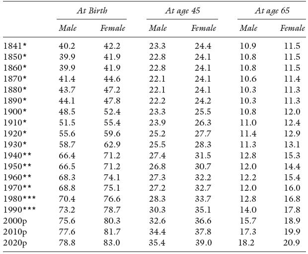
Notes: p = 2000-based population projections.
* Figures are based on English Life Tables.
** Figures are based on Abridged Life Tables.
*** Figures are based on future lifetime.

For England and Wales we see the gains in adult life expectancy in Table 3.4. An average man and women aged 45 years can expect to live 50 % longer than their mid–Victorian counterparts. While gains are still being registered by each new generation reaching retirement age, they have been small. Planning a pension scheme in the late 19th century was very different from that of today – more on this in Chapter Nine. The longer lives of those over 65 years of age, with current retirement ages, gives us the modern problem of increasing dependency of the elderly. In the US and elsewhere the gap between male and female life expectancy at birth increased through the 20th century only showing a convergence in the last two decades, see Figure 3.5. Failure of any pension scheme whether it is private or of government origin will be borne by the elderly single females of the population.

In the early 19th century, the English actuary/mathematician Benjamin Gompertz devised the law of mortality. In modern terms, this is a law of “system failure” that relates age and adult (post-reproductive age) death. The deaths are “all-cause” in that no particular cause is identified. It is an approximation, but one that fits very well for roughly the ages 25–35 to 80–90. The range of its accurate coverage will vary from one population to the next. Although it cannot be measured in history beyond about 100 years ago, it is thought to be generally applicable to older members of the population. The frequency of death rises geometrically with age, which is, of course, linear. To the Gompertz age-related algorithm, another 19th century actuary William Makeham added a non age-related term. Both Gompertz and Makeham were interested in the relationship between the frequency of death and age because of the usefulness of that prediction in the insurance industry. The Gompertz-Makeham approximation is thus the sum of the two separate arguments:

Law of Mortality: μ _x = A + B . c^x,

Where μ _x is the frequency of death at age x;

c is the coefficient of aging, c > 1

B is a constant, B > 0; and

A is background constant, non age-related rate of mortality, A ≥ -B.

Within the age range noted, the Gompertz-Makeham approximation has proven remarkably good at predicting death frequencies for relatively homogeneous populations. (Indeed, it has proven useful to estimate the deaths of various non-human populations from fruit flies to bacteria).

Two particular phenomena, themselves interesting, associated with death and age, limits the usefulness of the Gompertz-Makeham approximation over the entire lifespan. First, death rates at young ages are not well predicted essentially because they are not usually the result of regular system failure. Even although the death rates are high among the young, sometimes very high, they are brought about by non-age related events: poor nutrition, infection (or, perhaps, infectious diseases), disease, and so on. Second, for the very old there is actually a sudden deceleration of the μ _x term brought about by a change in the relationship between death and very old age. The reason, according to Shiro Horiuchi and John Wilmoth, is that healthier individuals appear selected by their physical characteristics to survive into very old age, so we end up with a non-representative group. It is also possible that at very old ages the rate of decay slows down – good news for some of us.³² For the age range between the limits the so-called intrinsic mortality (the system failure component of mortality) has not been fixed over time but has varied with:

lifestyle (superior nutritional and appropriate exercise choices);
pharmaceutical advances (insulin, for example); and
surgical advances and treatment protocols.³³

Figure 3.6 The Probability of Survival in History, ‘Rectangularization’.

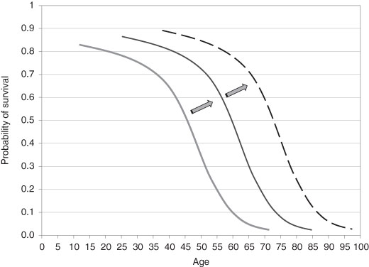
These of course are the results of growing income and of technological advances; income growth and technology are related, although not in a straightforward way, as we shall see later. The net result is that the intrinsic mortality has shifted over time and extended the age range over which the Gompertz-Makeham approximation holds true. (From the frequency of mortality at any given age we can compute the probability of death and its counterpart, the probability of not dying or survival.) The shift in the intrinsic mortality also changed the shape of the survival curve – the probability of not dying at any given age. The ugly but useful term of “rectangularization” describes how the curve shifts outward over time as the effects operate.³⁴ How these have changed over history is given in Figure 3.6.

The background non-age related mortality pattern has also changed over time and, although this has had a positive effect in recent times, as economic historians we cannot assume that this has always been so. Distinctions may be made in the survival curve: by gender, by time, and by location. For instance, there was (is) a higher rate of death for older males compared to the similar cohort of females. This is expressed in the much longer life expectancy at age 60 for females in western and Asian countries. While the basis of this shorter life for males is not well understood, it is likely that there are both biological and economic reasons. The current age expectancy gap has shown a decline in recent years in most OECD countries. This has led to speculation that as women face less arbitrary discrimination in labor markets (and their working lives become more like those of men) they will tend to have similar mortality patterns. This supposes that a key element in separating the genders is workplace stress. The reduction of the gap is brought about by the rise of the male life expectancy relative to that of the females.³⁵ However, female life expectancies are still, and have been throughout history, greater than males. There have been direct economic consequences of this: single, elderly women are usually amongst the poorest groups in society – more in Chapter Seven. It has always been so.

3.4 Seasonal Pattern of Death

The anthropological evidence suggests that, when humankind moved into settled communities associated with agriculture, the mortality rate rose. This, as noted before, was brought about by the increased contact with disease pathogens due to the proximity of domesticated fowl and livestock. Furthermore, the density within the habitations was increasing thereby creating an environment for the effective spread of disease among the families who lived there. In addition, housing was frequently shared with domestic animals – they were a welcome source of heat. The houses were usually closely arranged in a village or town pattern. Most early farming was conducted with people living in villages venturing out to tend their land holdings. The result was that disease spread rapidly from one family to another. Even when individual farms were created separately from a village, the underlying cause of disease spread did not diminish much. Of course, the economic issue is why did humankind choose to farm with social arrangements that seemed to maximize the mortality rate? First, there was no knowledge of disease and the nature of its spread. To the people involved, the disease pools created by sedentary farm life were an unintended, and not understood, consequence of the arrangements. Second, the new social arrangements certainly created benefits that reduced the variability of supply. Villages provided insurance as defence against incursions and threat to the sedentary farm system. Third, common-field holding, with widely separated plots and fields, spread the ownership or entitlement over the geography and, thus, was a method of risk-sharing: the risk of flooding, of poor soil quality, or other natural calamities.

The time pattern of mortality over the year followed a regular cycle. However, the seasonal pattern was different in the rural areas from that in the towns and cities. In the farming areas, it was coincident with the annual farm cycle. Deaths were low in the late summer and autumn. This is the period of the year when food is most abundant. Food was relatively plentiful even in the early winter because of the end of season slaughter of animals. However, in the late winter and early spring, inventories of food ran down, and in a bad year might be exhausted, and death rates rose to their highest for the year:

Food became less abundant (and more expensive), and malnutrition increased in severity and occasionally there was starvation.
Insufficient household heating and inadequate clothing made weakened people vulnerable to infections.
In colder climates with both people and animals kept indoors longer there was an increase the exposure to disease pools.

Death rates remained high in the spring and early summer (peak mortality was in April/May depending on the location) and then fell dramatically as fresh food appeared as the weather warmed. Thus we find the same seasonality in 17th century England as in farming areas throughout north-western Europe (and probably also in North America).³⁶ This variability moderated over the course of the “long 18th century.”³⁷ By the middle of the 1800s, nonetheless, rural mortality still showed greater seasonal variation than that of the towns and cities.³⁸ This does not mean that mortality was lower in urban areas and higher in rural areas, it was not. Woods estimates that the life chances were, in general, 1.5 times greater in the rural areas (measured in terms of life expectancy).³⁹ Throughout the 19th century, as agricultural income variability fell, the extreme variability of the annual mortality cycle moderated (extraordinary events such as the Irish Famine of the 1840s notwithstanding – see Chapter Five).

Figure 3.7 Urban Mortality in London by Month, 1670 and 1800.

Source: data from Landers and Mouzas (1998).

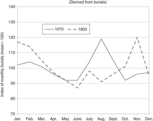
Well into the 20th century annual urban mortality was generally greater than rural mortality and sometimes very much greater. Urban areas also experienced seasonal variation of mortality, but a different one from the rural areas. In the pre-modern period (before c.1800) the peak in the death rates over the year generally occurred in late summer. (Rural mortality in late summer was at a seasonal low). The deaths during the peak were mostly from diseases that were water borne. They disproportionately affected the very young. A new peak emerged in absolute terms – see Figure 3.7 – in the late autumn and early winter to about February.⁴⁰ However, by the late 19th century in most areas of Western Europe and North America, this peak had largely disappeared. Since this was well before the large social investment in sewage systems and clean water supplies, researchers have hypothesized that there was either an exogenous change in the virulence of some of the water borne disease pathogens or a change in the environment in which they thrived. Perhaps both conditions held.

The extreme nature of the seasonal peaks fell in both rural and urban mortality began to moderate in the late 19th/early 20th centuries along with the fall in the annual mortality toll in western countries. Yet, there the rural-urban difference had proven remarkably persistent for a long time.

3.5 Seasonality and Longevity

For those born before World War II, the season of their birth was an important predictor of longevity. The theory behind this unexpected finding is the much-debated “fetal origins hypothesis” of David Barker and others.⁴¹ They argue that malnutrition at very young ages, including in utero, influenced morbidity and mortality later in life. Low birth weights were associated with maternal malnutrition, and this contributes to greater morbidity at older ages from cardiovascular disease, hypertension, and type 2 diabetes. In addition, maternal infections from diseases such as tuberculosis impaired fetal growth. The nutrition and infection explanations are complementary mechanisms tying morbidity in early and later life.⁴² Both have found empirical support.⁴³

In the Northern Hemisphere, mortality at age 50 and over was higher for those born in the spring and lower for those born in the autumn. In the Southern Hemisphere, the pattern was reversed, as are the seasons. The difference in life span between peak and trough ranged from 0.6 years in Austria and Australia to 0.3 years in Denmark. The number for the US was 0.4 years, but with considerable regional variation as might be expected. New England (0.31 years) and the Middle Atlantic (0.36 years) were much lower than the East South Central (0.86 years) and the West South Central (0.69 years).⁴⁴ One expects the US South to have been less healthy because of the greater proportion of fried foods in that diet and a higher incidence of infectious diseases, parasitic diseases, and gastroenteritis.

Before World War II, the influences of both nutrition and infection were highly seasonal. The typical diet in the early years of the 20th century was different from that at the beginning of the 21st century. The availability and prices of fresh fruits and vegetables varied over the year, and people ate less of them. People ate less meat and more starch. Nutritionists even argued that green vegetables demanded more energy for digestion than they supplied. The nutrition explanation has more to do with the quality and variety of the food available, especially during the winter and spring, than its quantity. Although severe malnutrition was limited in all the countries studied, there was inadequate nutrition in those days during the winter and early spring. Since a fetus has its greatest weight growth during the third trimester, Northern Hemisphere infants born in the spring spent their third trimester in utero during a period of relatively poor nutrition, while the opposite was true for infants born in the fall.

The incidence of infectious disease depends on the climate and on the seasons of the year. Gastrointestinal infections were more common in summer; there was (and is) a correlation between the incidence of water- and food-borne infectious diseases and warmer temperatures. In the late 19th century, the movement of non-pasteurized milk without adequate refrigeration contributed to many ailments including gastroenteritis, a major contributor to the infant mortality rate.⁴⁵ Respiratory infections (airborne diseases), spread in poorly ventilated conditions, were more common in autumn and winter. Current research cannot distinguish between the period in utero and the first year of life. Thus, we cannot determine whether mother’s nutrition during pregnancy or infectious disease in the first year of life is of crucial importance. It is the case, however, that before World War II, Northern Hemisphere babies born in the spring experienced a transition from a period of less adequate nutrition to one of more infection. The opposite was true for those born in the fall, and the pattern was reversed for Southern Hemisphere babies.

3.6 Urban Mortality

Before 1900, urban mortality was substantially higher than rural mortality in both Europe and North America, particularly for infants and children. Even the earliest of systematic research, in the late 19th century, reported that life expectancy at birth in Massachusetts cities was almost seven years less than that in the state as a whole.⁴⁶ There are numerous reasons proffered for the higher urban mortality rates. Urbanization and industrialization were co-temporal. The need to ship food from farm to city in the age before refrigeration meant that urban food supplies were less healthy. The large numbers of people moving into the cities meant that new diseases arrived daily, and the large numbers of people living in close quarters meant that disease transmission was easy.⁴⁷

In 1900 the US Bureau of the Census created the Death Registration Area (DRA), which included ten states and the District of Columbia. The DRA rates were based on the registration of deaths shortly after they occurred; the Bureau’s Census of Mortality rates (which date from 1850) are the result of the enumerator asking how many deaths had occurred the previous year.⁴⁸ The Bureau’s initial estimates using the DRA were that life expectancy at birth in 1901 was ten years less for white males born in cities than for those born in rural areas; for white females, the difference was about seven years. There are, however, several problems with the original DRA data. In particular, it covered only 26.3 % of the US population and, more importantly, the areas were ones in which urban and foreign residents were over-represented, and blacks were under-represented. Consequently, using the DRA information, the overall US mortality was overestimated by failure to recognize the urban distinctiveness.⁴⁹

The US Census Bureau itself also became aware of the rural-urban differences in mortality and conducted a number of regional studies. In 1942 one important study compiled a historical life table for urban and rural areas in 1830.⁵⁰ It revealed that life expectancy at age ten was:

51 years in 46 small New England towns (mostly in Massachusetts);
46 years in Salem, MA (pop. 14 000) and New Haven, CT (11 000); and
about 36 years in New York City (203 000), Philadelphia (80 000), and Boston (61 000).

Thirty years later these results were criticized for confusing urban-rural differences in longevity with regional disparities in mortality.⁵¹ Deaths in smaller towns, it was claimed, were likely to have been under-registered and subsequent corrections reduced the difference somewhat.⁵²

Similar disparities in urban and rural mortality were discovered in Europe. David Glass found life expectancy at birth in England and Wales in 1841 to be 40.2 years for males and 42.2 years for females. However, life expectancy in London was only 35 years for males and 38 years for females, and the numbers were even lower for the industrial cities of Manchester and Liverpool.⁵³ On the continent, between 1816 and 1820 female life expectancy at birth in the département of the Seine, that included Paris, was 30.83 years, more than eight years below that of France as a whole.⁵⁴ The gap then widened to ten years in 1851–1855 before falling to eight years in 1876–1880 and to 4.6 years in 1901–1905. This was similar to Germany in 1900–1901 where male life expectancy at birth was about four years lower in urban than in rural areas, but female was only about a year and a half lower.⁵⁵

In the late 19th century, most differences in urban and rural mortality were due to differences in infant and child mortality.⁵⁶ This was due primarily to infectious diseases, whose incidence was influenced by living standards and improvements in public health, particularly water and sewer systems.⁵⁷ The US Children’s Bureau reported that the difference between rural and urban infant mortality rates was nine per 1000 at 1915 but fell to just over one per thousand by 1921. As late as 1939 statisticians for the Metropolitan Life Insurance Company calculated that rural mortality rates remained lower than urban mortality rates, although the disparity between cities of different sizes had essentially disappeared.⁵⁸ From a longer perspective, the infant mortality rate in English cities with more than 100 000 inhabitants was 42 % higher than in rural areas in the 1850s but the gap had widened to 46 % by the early 1900s.⁵⁹

While the difference was smaller in certain parts of continental Europe this has been attributed to higher infant mortality rates in both German cities and rural areas than elsewhere.⁶⁰ In Germany, 1875–1877, the infant mortality rate was only 10 % higher in urban areas than in rural areas and the same was roughly true of the Netherlands in the late 19th century.

There have been five explanations offered for the upward trend in the urban-rural difference in the 19th century and the decrease in the 20th century. These five are: improvements in the standard of living, improvements in medical science, advances in sanitation systems, improvements in the fluid milk supply, and changes in migration patterns.

Improvements in the Standard of Living. In a series of articles culminating in his book, Thomas McKeown (1976) holds that improvements in nutrition were primarily responsible for the increase in life expectancy occurring during the 19th century. Although many have challenged McKeown’s emphasis on the role of nutrition over all other factors in the decrease in mortality, none deny that nutrition was a factor.⁶¹ The nutrition hypothesis can explain why urban mortality would exceed rural mortality in two ways. First, rural residents, who tended to be farmers or farm workers, had better access to cheaper and healthy food. Second, although average incomes tended to be higher in cities, personal income inequality tended to be lower in rural areas.⁶² This suggests that cities had a higher proportion of residents living in poverty, without adequate access to nutrition and that areas or individuals with lower incomes or socioeconomic status had higher mortality.⁶³

Improvements in the Science of Medicine. Advances in medical science contributed substantially to the decline in mortality, particularly in urban areas. The most important development was the acceptance of the germ theory of disease by both the medical profession and the public. Before 1880, the dominant theory was the miasmatic theory: foul odors released by decomposing matter caused disease. In some cases (e.g., better ventilation and clean streets) the older theory led cities to do the right thing for the wrong reason, but other actions (e.g., as an undue emphasis on the dangers of sewer gas) were cosmetic at best. As Nancy Tomes pointed out, it was the germ theory, with its emphasis on preventing the spread of harmful bacteria that led to measures such as water filtration and chlorination, the scientific testing of water and food for contaminants, and public health campaigns against such leading causes of death as tuberculosis and infantile diarrhoea.⁶⁴ Further, the application of proper sanitary techniques within the home greatly reduced the spread of infectious disease.⁶⁵ Since these public and private innovations were generally applied sooner in urban than in rural areas, urban mortality declined faster in the late 19th and early 20th centuries than rural mortality. On the other hand, McKeown is probably correct in arguing that advances in medical practice did little to reduce mortality before World War I as these were limited primarily to the development of sterile surgical techniques, inoculation and vaccination for smallpox, and an antitoxin for diphtheria.

Advances in Sanitation Systems. McKeown, however, underestimates the effect of public health measures. The great reduction in the incidence of waterborne diseases, such as cholera and typhoid fever, which these public health innovations brought about also greatly reduced mortality from airborne diseases by improving the quality of nutrition and reducing other insults to the body.⁶⁶ The provision of clean water was responsible for almost half of the total mortality reduction occurring in cities during the early 20th century, including three-quarters of the fall in infant and two-thirds of the decline in child mortality.⁶⁷ Expenditures on sewer systems and refuse collection and disposal significantly reduced cities’ mortality rates from waterborne disease, but expenditures on water systems were less effective, with the exception of cities drawing their water supplies from rivers.⁶⁸ The provision of potable water, however, was one of the first major public health innovations and was largely in place so the incremental expenditures had a smaller mortality payoff in the late 19th/early 20th century. A fall in the mortality rate from typhoid, a waterborne disease, a proxy for water quality, was associated with a significant fall in the mortality rate from pneumonia, which was not a waterborne disease.⁶⁹ This supports the Mills-Reincke phenomenon: as cities began to filter their water supplies, death rates from non-waterborne diseases often declined in greater proportion than did death rates from water-borne diseases. Much of the variation in mortality in three French départements in the 19th century could be explained by differences in the quality of the water and sewer systems.⁷⁰ In Chicago, the provision and improvement of the public water supply lowered the city’s mortality rate between 35 and 56 % from 1850 to 1925, a result attributable primarily to eradicating typhoid.⁷¹

Improvements in the Milk Supply. Closely aligned with public health improvements were improvements in the quality (and quantity) of the milk supply. These improvements reduced excessive infant mortality in the cities, particularly during the summer months – see earlier. In the mid-19th century, urban-rural disparities in infant mortality widened as cities began to import milk over longer distances, often under unsanitary conditions. The greater relative anonymity of sellers also led to the adulteration of milk and the sale of “swill milk” that had been collected from cows fed on the by-products of distilleries. Over the course of the late-19th and early-20th centuries numerous changes were made. Milk was tested, first for adulteration and later for bacteria content, and regulations were adopted regarding the handling and sale of raw milk. In particular, laws were passed requiring pasteurization and attempts were made to eradicate bovine tuberculosis. There were public education campaigns encouraging breastfeeding or the use of safe milk. First iceboxes and later refrigerators in the home kept milk from spoiling. Finally, in some cities, safe milk was distributed at subsidized prices to mothers in urban slums, where infant mortality rates were extremely high.⁷² In both Europe and North America, the home delivery of milk gained popularity in the early 20th century.

Changes in Migration Patterns. A final explanation for the pattern of urban-rural mortality rates is that large waves of internal and international migrants to urban areas increased the incidence of infectious diseases. Diverse groups of people who previously had not been exposed to one another’s diseases came into contact with each other under crowded conditions. Foreign migrants, in particular, were vulnerable because of the stresses associated with the transatlantic passage. An increase in migration in the late 19th century significantly increased the crude death rate in large American cities.⁷³ Earlier, in 1850, according to an extensive study, any location that had access to regional transportation networks via a water route significantly increased the exposure of its resident population to the higher mortality associated with the volume of internal and international migrants.⁷⁴ Yet, this cannot explain the fact urban mortality declined more rapidly than rural mortality in the late 19th century. Any negative effects of immigration on mortality had to have been offset by something like the effects of improvements in living standards and public health.

The study of past urban-rural mortality differentials and the burden of disease have particular relevance for the developing world today.⁷⁵ Not only are diseases such as malaria and tuberculosis still common in the developing world, but urbanization is proceeding there at an increasing pace. Of the 31 cities worldwide that have populations over 5 million, 25 are located in the developing world.

3.7 The Mortality Transition: Crude Death Rates

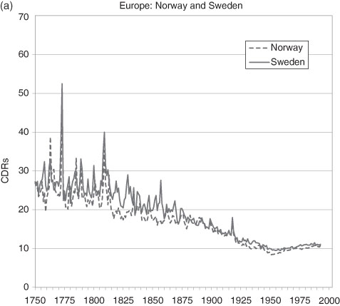
The slow pre-1800 decline in the crude death rate gathered momentum and, in Western Europe, by the late 19th century had travelled about half the distance of the transition (Figure 3.8). There were yet gains to be made, as noted earlier, the most significant of which were in the first half of the 20th century. Variations in country performance are largely explained by the different degrees of urbanization, the amount of spending of social infrastructure and local improvements in the standard-of-living. But not only did the CDR decline to its modern level, its variance also declined. Apart from human inspired catastrophes such as wars and their spillover effects, since the great influenza pandemic of 1919 Western Europe and North America have been spared (and taken pre-emptive measures to limit) major afflictions which move the national mortality rate significantly. There are of course many life-saving gains in the future from appropriate medical and drug therapies, social investment and poverty relief that might be expected. The AIDS/HIV epidemic, and others, have smaller aggregate effects than the great scourges of pre-20th century history: smallpox, cholera, influenza, typhus, polio, scarlet fever and many others. The same is not true of the less developed world, as has been noted.⁷⁶

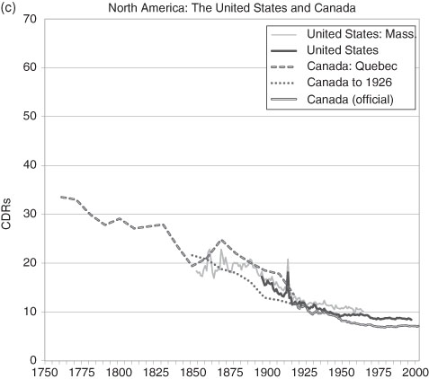
For the US, the aggregate CBR is available only for the years after 1900 due to the way the national census was constructed. With this deficiency over a crucial period, the state records for Massachusetts fill in the broad picture of the 19th century from 1855 onward.⁷⁷ In general terms, there is no reason why the state’s CDR should vary significantly from the national one. It of course would be higher than the unobserved national CDR because of the higher rate of urbanization in the state relative to the nation. For aggregate statistics we cannot go further into the past with direct evidence. Yet, for Canada we can. The records of mortality are remarkably complete for the Roman Catholic population of Quebec so that a CDR can be calculated.⁷⁸ We might argue that there is no major distinction (there are many minor ones) between the demography of New France/Quebec and that of the other British North American colonies during the US Colonial Era and little thereafter that are not accounted for by measurable population differences such as the rural-urban mix.⁷⁹ (Quebec is contiguous to the US and shared similar economies with the New England states.) A reasonable inference is that the earlier stages of the US demographic transition can be mirrored by the Canadian data. Certainly by the year that the US (Massachusetts) data begins the CDRs in the US and Canada/Quebec are roughly equal. So, the US in 1800 would be estimated to have had a CDR similar to that of Canada and North Western Europe, somewhat below 30 per 1000.

The next task is to account for the long run decline in the fertility rate. Key to understanding this is the question: what was the relationship between mortality and natality – measured by the crude death and birth rates respectively?

Note: Data for England to 1838 from Wrigley and Schofield (1981) and Official Estimates for England and Wales thereafter. The French data prior to 1801 are from Bourgeois-Pichat (1965); they are interpolated from five year averages. “W-S” refers to the “Wrigley-Schofield estimates”.

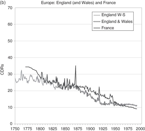
Figure 3.8 Crude Death Rates in Western Europe and North America, 1750 to the Present.

Sources: Bourgeois-Pichat (1965); Haines (2006), US Historical Statistics, Series Ab 988 and Ab1048; Henripin and Peron (1972); Historical Statistics of Canada, Series B18; Mitchell, International Historical Statistics, Series, 93–117; Statistics Canada (various) including Canadian Census data; US Census data; and Wrigley and Schofield (1981).

Note: Data prior to 1880 for Quebec are for the Roman Catholic population only. All data prior to 1921 are interpolated for the ten year census intervals. Between 1976 and 1998 the data are interpolations for the five year census intervals. The US data are for all individuals; where no national figures exist, historians use the CDR of the State of Massachusetts.

Endnotes

1 Children under 12 months of age. World Health Report for 2005, http://www.who.int/whr/2005/en/index.html

2 Omran, (1971) and Salomon and Murray (2002).

3 Bacci (1991).

4 The Horn of Africa (Somalia. parts of Ethiopia, Sudan, Eritrea) provides startling examples of the near total paralysis of the food distribution system. Even the UN and other charitable agencies are frequently frustrated in their efforts to provide relief.

5 Infectious and parasitic diseases: Tuberculosis; STIs excluding HIV (Syphilis, Chlamydia Gonorrhoea); HIV/AIDS; Diarrhoeal diseases; Childhood diseases (Pertussis, Poliomyelitis, Diphtheria, Measles, Tetanus); Meningitis; Hepatitis; Malaria; Tropical diseases (Chagas disease, Schistosomiasis, Leishmaniasis, Lymphatic filariasis, Onchocerciasis) Leprosy; Japanese encephalitis, Trypanosomiasis Trachoma); Intestinal nematode infections (Ascariasis, Trichuriasis, Hookworm disease); Respiratory infections (Lower and Upper respiratory infections incl. Otitis media).

6 Drug resistant strains of Mycobacterium tuberculosis and Mycobacterium bovis give rise to the fear that the incidence of tuberculosis may again rise.

7 Centers for Disease Control and Prevention (Nov., 1999), “The Deadly Intersection Between TB and HIV”, Bulletin, Department of Health and Human Services, US Government – http://www.cdc.gov

8 Ubelaker (2000).

9 Ellman and Maksudov (1994), Table 1. The figure was arrived at taking the estimated total deaths minus the recent estimate of military deaths (22.6–8.7 millions). See also: Haynes (2003).

10 For very low rates of mortality, it is sometimes expressed per 10 000.

11 Notice that these rates are inclusive but it is essential to check the exact definition for each study since sometimes they are not. For example, child mortality is often measured as 1–4 years.

12 Ó Gráda (2004).

13 UN, Statistics Division … 1.

14 Dzakpasu, Kramer, and Allen (2000).

15 Tropical diseases were not of course prevalent in northern hemisphere countries.

16 Based on the backward projections; Woods (1997). Schellekens (2001).

17 See Chapter Two.

18 Woods (1997).

19 Haines (1985).

20 For a discussion see: Perrenoud (1984). For the US see: Vinovskis (1972), 184–213 and for England and Wales see: Wrigley and Schofield (1981).

21 Bourbeau, Légaré and Émond (1997).

22 See Chapter Three for a discussion of CBRs and sustainability.

23 Hielte (2004).

24 We cannot reject the possibility that the data are not comparable.

25 Perrenoud (1984), Table 7.

26 Högberg (2004); Sundin (1995); Fridlizius (1984).

27 Vinoviskis (1971). Vinovskis argues that Wigglesworth adjusted his estimates of a lower calculation by methods that cannot now be duplicated and treats this figures as a plausible, well-educated guess.

Life expectancy at birth	1850	1900
white males	37.2	47.1
white females	39.4	48.4

Haines and Avery (1980), “The American Life Table of 1830–1860…”, Haines (2006), “Vital Statistics,” U.S. Historical Statistics, chapter Ab. Life tables for “All Races” and “Non-Whites” are available from 1900 onward.

29 Data from Perrenoud (1984), Table 7; Fridlizius (1984).

30 “Old” is a subjective notion. Human rights legislation in many world jurisdictions now forbids age discrimination, such as mandatory retirement.

31 Horiuchi and Wilmoth (1998).

32 Olshansky and Carnes (1997); Kesteloot and Huang (2003).

33 Wilmoth and Horiuchi (1999).

34 For instance, see: UK (2008), Health Expectancy, National Statistics. http://www.statistics.gov.uk

35 Wrigley and Schofield (1981).

36 The long 18th century refers to the period between the radical change in government in the United Kingdom in 1689 – the Glorious Revolution – and the fall of Napoleon at Waterloo in 1815.

37 Hayward, Pienta and McLaughlin (1997).

38 Evidence from: Jonsson (1984).

39 Woods (2003).

40 One of the reasons that researchers cannot be more precise is that the most frequently found evidence, the bills of mortality, did not give information that conformed to modern medical diagnoses of disease.

41 See, for example, Barker (2002).

42 Finch and Crimmins (2004).

43 Doblhammer (2003); see also Ferrie, Rolf and Troesken (2007).

44 Doblhammer (2003).

45 See Lee (2007).

46 Weber (1899).

47 New York (2007).

48 Higgs (1979); Condran and Crimmins (1980).

49 Preston and Haines (1991); Haines (1977).

50 Vinovskis (1972) gives a critique of the early life tables.

51 Ibid. Life expectancy at ages 10–14 in Massachusetts towns with less than 1000 inhabitants was estimated to be 52.5 years but 46.7 years in towns with 10 000 or more inhabitants.

52 A number of other demographers have calculated large disparities between rural and urban mortality rates. See Condran and Crimmins (1983), Haines (1977), Higgs (1973), Yasuba (1962), and Dublin and Lotka (1945).

53 Glass (1973). See also Szreter and Mooney (1998).

54 Preston and van de Walle (1978).

55 Vogele (1998).

56 Kunitz (1983).

57 Duffy (1990); McKeown and Record (1962); McKeown (1976); Melosi (2000); and Preston and Haines (1984).

58 Woodbury (1926).

59 Williams and Galley (1995); see also Huck (1995) and Woods, Watterson, and Woodward (1988).

60 Williams and Galley (1995) and van Poppel, Jonker, and Mandemakers (2005).

61 Szreter (1988); Riley (1990) and Woods (2003).

62 McLaughlin (2002).

63 Among the studies that provide evidence for this are Steckel (1988); Condran and Cheney (1982); Crimmins and Condran (1983); Haines (1995); Woods, Watterson; and Woodward (1988).

64 Tomes (1998).

65 Both Tomes (1998) and Mokyr (2000) point out this could be overdone.

66 Harris (2004).

67 Cutler and Miller (2005).

68 Cain and Rotella (2001). See also Gaspari and Woolf (1985).

69 Condran and Crimmins (1983). Condran and Cheney (1982) found evidence that water filtration reduced the incidence of mortality from typhoid, but they found no evidence that it reduced infant and child mortality rates from diarrhoeal diseases; both had been declining for at least 20 years before filtration.

70 Preston and van de Walle (1978).

71 Ferrie and Toesken (2008).

72 See Beaver (1973); Meckel (1990a and b); Lee (2007); and Olmstead and Rhode (2004).

73 Higgs (1979) study of 18 US cities.

74 Haines, Craig and Weiss (2003) using data from over 1200 US counties in 1850.

75 Riley (1990, 2005).

76 Ó Gráda (2004).

77 See Haines (2006) and Zopf Jr. (1992).

78 Henripin and Peron (1972). Quebec refers to New France (1765–1790), Lower Canada (1791–1840), Canada East (1841–1867) and Quebec thereafter.

79 Infant mortality was notably different between the French and English speaking Quebecers of the late 19th and early 20th century. This too can be largely attributed to the rural and urban differences of the two groups.

References

Bacci, Massimo Livi (1991) Population and Nutrition: An Essay on European Historical Demography, Cambridge: Cambridge University Press.

Barker, David J.P. (2002) “Fetal Programming of Coronary Heart Disease,” Trends in Endocrinology & Metabolism, 13(9), 364–8.

Beaver, M.W. (1973) “Population, Infant Mortality and Milk”, Population Studies, 27(2), 243–54.

Bengtsson, Tommy, Gunnar Fridlizius and Rolf Ohlsson (eds.) (1984) Pre-Industrial Population Change: The Mortality Decline and Short-Term Population Movements, Stockholm: Almquist and Wiksell International.

Bourbeau, Robert, Jacques Légaré and Valérie Émond (1997) New Birth Cohort Life Tables for Canada and Quebec, 1801–1991, Ottawa: September, Statistics Canada, Catalogue No. 91F0015MPE.

Bourgeois-Pichat, J. (1965) “The General Development of the Population of France Since the Eighteenth Century”, in D.V. Glass and D.E.C. Eversley, eds. Population in History, Essays in Historical Demography, Old Woking, Surrey: Edward Arnold Publishers.

Cain, Louis P. and Elyce J. Rotella (2001) “Death and Spending: Urban Mortality and Municipal Expenditure on Sanitation”, Annales De Demographie Historique, 1, 139–54.

Condran, Gretchen A. and Rose A. Cheney (1982) “Mortality Trends in Philadelphia: Age- and Cause-Specific Death Rates 1870–1930”, Demography, 19(1), 97–123.

Condran, Gretchen A. and Eileen M. Crimmins (1983) Mortality Variation in U.S. Cities in 1900: A Two-Level Explanation by Cause of Death and Underlying Factors”, Social Science History, 7(1), 31–59.

Cutler, David and Grant Miller (2005) “The Role of Public Health Improvements in Health Advances: The Twentieth-Century United States”, Demography, 42(1), 1–22.

Doblhammer, Gabriele (2003) “The Late Life Legacy of Very Early Life,” Max Planck Institute for Demographic Research Working Paper WP 2003–030, September.

Dublin, Louis I. and Alfred J. Lotka (1945) “Trends in Longevity” Annals of the American Academy of Political and Social Science, 237, World Population in Transition, 123–33.

Duffy, John (1990) The Sanitarians. Urbana, IL: University of Illinois Press.

Dzakpasu, Susie, K.S. Joseph, Michael S. Kramer and Alexander C. Allen (2000) “The Matthew Effect: Infant Mortality in Canada and Internationally”, Pediatrics, 106(1), e1–5.

Ellman, Michael and S. Maksudov (1994) “Soviet Deaths in the Great Patriotic War: A Note” Europe-Asia Studies, 46(4), 671–80.

Ferrie, Joseph and Werner Troesken (2008) “Water and Chicago’s Mortality Transition, 1850–1925,” Explorations in Economic History, 45(1), 1–16.

Ferrie, Joseph, Karen Rolf and Werner Troesken (2007) “The Past as Prologue: The Effect of Early Life Circumstances at the Community and Household Levels on Mid-Life and Late-Life Outcomes,” Working Paper, January.

Finch, Caleb E. and Eileen M. Crimmins (2004) “Inflammatory Exposure and Historical Changes in Human Life-Spans,” Science, 305(17), 1736–9.

Fridlizius, Gunnar (1984) “The Mortality Decline in the First Phase of the Demographic Transition: Swedish Experiences”, in Bengtsson et al., 71–109.

Gaspari, K. Celeste and Arthur G. Woolf (1985) “Income, Public Works, and Mortality in Early Twentieth-Century American Cities Income, Public Works, and Mortality in Early Twentieth-Century American Cities”, Journal of Economic History, 45(2), 355–61.

Glass David V. (1973) Numbering the People: the Eighteenth-Century Population Controversy and the Development of Census and Vital Statistics in Britain, Farnborough: D.C. Heath.

Haines, Michael (1995) “Socio-economic Differentials in Infant and Child Mortality during Mortality Decline: England and Wales, 1890–1911”, Population Studies, l. 49(2), 297–315.

Haines, Michael R. (1977) “Mortality in Nineteenth Century America: Estimates From New York and Pennsylvania Census Data, 1865 and 1900”, Demography, 14(3), 311–31.

Haines, Michael R. (1985) “Inequality and Childhood Mortality: A Comparison of England and Wales, 1911, and the United States, 1900”, Journal of Economic History, 45(4), 885–912.

Haines, Michael R. (1989) “American Fertility in Transition: New Estimates of Birth Rates in the United States, 1900–1910”, Demography, 26(1), 137–48.

Haines, Michael R. (2006) “Vital Statistics, Chapter Ab”, U.S. Historical Statistics.

Haines, Michael R. and Roger C. Avery (1980) “The American Life Table of 1830–1860: An Evaluation”, Journal of Interdisciplinary History, 11(1), 73–95.

Haines, Michael R., Lee A. Craig and Thomas Weiss (2003) “The Short and the Dead: Nutrition, Mortality, and the “Antebellum Puzzle” in the United States”, Journal of Economic History, 63(2), 382–413.

Harris, Bernard (2004) “Public Health, Nutrition, and the Decline of Mortality: The McKeown Thesis Revisited”, Social History of Medicine, 17(3), 379–407.

Haynes, Michael (2003) “Counting Soviet Deaths in the Great Patriotic War: A Note” Europe-Asia Studies, 55(2), 303–9.

Hayward, Mark D., Amy M. Pienta and Diane K. McLaughlin (1997) “Inequality in Men’s Mortality: The Socioeconomic Status Gradient and Geographic Context”, Journal of Health and Social Behavior, 38(4), 313–30.

Henripin, J. and Y. Peron (1972) “The Demographic Transition of the Province of Quebec”, in D.V. Glass and Roger Revelle (eds.), Population and Social Change, London: Edward Arnold, 213–31.

Hielte, Maria (2004) “Sedentary Versus Nomadic Life-Styles: The ‘Middle Helladic People’ in Southern Balkan (late 3rd & first Half of the 2nd Millennium BC)”, Acta Archaeologica 75, 27–94.

Higgs, Robert (1973) “Race, Tenure, and Resource Allocation in Southern Agriculture, 1910”, Journal of Economic History, 33(1), 149–69.

Higgs, Robert and David Booth (1979) “Mortality Differentials within Large American Cities in 1890”, Human Ecology, 7(4), 353–70.

Högberg, Ulf (2004) “The Decline in Maternal Mortality in Sweden: The Role of Community Midwifery”, American Journal of Public Health, 94(8) (Spring), 1312–20.

Horiuchi, Shiro and John R. Wilmoth (1998) “Deceleration in the Age Pattern of Mortality at Older Ages”, Demography, 35(4), 391–412.

Huck, Paul (1995) “Infant Mortality and Living Standards of English Workers During the Industrial Revolution”, Journal of Economic History, 55(3), 528–50.

Jonsson, Ulf (1984) “Population Growth and Agrarian and Social Structure: Some Swedish Examples”, in Bengtsson et al., 223–54.

Kesteloot, H. and X. Huang (2003) “On the Relationship between Human All-Cause Mortality and Age”, European Journal of Epidemiology, 18(6), 503–11.

Kunitz, Stephen J. (1983) “Speculations on the European Mortality Decline”, Economic History Review, New Series, 36(3), 349–64.

Landers, John and Anastasia Mouzas (1998) “Burial Seasonality and Causes of Death in London 1670–1819”, Population Studies, 42(1), (March), 59–83.

Lee, Kwang-sun (2007) “Infant Mortality Decline in the Late 19th and Early 20th Centuries: The Role of Market Milk,” Perspectives in Biology and Medicine, 50(4), 585–602.

McKeown, T. (1976) The Modern Rise of Population, London: Edward Arnold.

McKeown, T. and R.G. Record (1962) “Reasons for the Decline of Mortality in England and Wales during the Nineteenth Century”, Population Studies, 16(2), 94–122.

McLaughlin, Diane K. (2002) “Income Inequality in America: Nonmetro Income Levels Lower Than Metro, But Income Inequality Did Not Increase as Fast”, Rural America, 17(2), 14–20.

Meckel, Richard A. (1990a) “ Immigration, Mortality, and Population Growth in Boston, 1840–1880”, Journal of Interdisciplinary History, 15(3), 393–417.

Meckel, Richard A. (1990b) Save the Babies. American Public Health Reform and the Prevention of Infant Mortality, 1850–1929, Baltimore: Johns Hopkins University Press.

Melosi, Martin V. (2000) The Sanitary City: Urban Infrastructure in America from Colonial Times to the Present, Baltimore: Johns Hopkins University Press.

Mokyr, Joel (2000) “Why ‘More Work for Mother?’ Knowledge and Household Behavior, 1870–1945”, Journal of Economic History, 60(1), 1–41.

New York City (2007) Summary of Vital Statistics 2006 for the City of New York, Bureau Of Vital Statistics, New York: New York City Department Of Health And Mental Hygiene. http://www.nyc.gov/html/doh/html/vs/vs.shtml

Ó Gráda, Cormac (2004) “Infant and Child Mortality in Dublin a Century Ago“, Marco Bresci and Lucia Pozzi (eds.), The Determinants of Infant and Child Mortality in Past European Populations, (Forum, Italy: Udine), 89–104.

Olmstead, Alan L. and Paul W. Rhode (2004) “An Impossible Undertaking: The Eradication of Bovine Tuberculosis in the United States”, Journal of Economic History, 64(3), 734–72.

Olshansky, S. Jay and Bruce A. Carnes (1997) “Ever Since Gompertz”, Demography, 34(1), 1–15.

Omran, A. (1971) “The Epidemiological Transition: A Theory of the Epidemiology of Population Change”, Milbank Memorial Fund Quarterly, 49, 509–38.

Perrenoud, Alfred (1984) “Mortality Decline in Its Secular Setting”, in Bengtsson et al., 41–69.

Preston, Samuel H. and Michael R. Haines (1984) “New Estimates of Child Mortality in the United States at the Turn of the Century”, Journal of the American Statistical Association, 79(386), 272–81.

Preston, Samuel H. and Etienne van de Walle (1978) “Urban French Mortality in the Nineteenth Century”, Population Studies, 32(2), 275–97.

Riley, James C. (1990) “The Risk of Being Sick: Morbidity Trends in Four Countries”, Population and Development Review, 16(3), 403–32.

Riley, James C. (2005) “The Timing and Pace of Health Transitions around the World”, Population and Development Review, 31(4), 741–64.

Salomon, J.A. and C.J.L. Murray (2002) “The Epidemiologic Transition Revisited: Compositional Models for Causes of Death by Age and Sex”, Population and Development Review, 28, 205–28.

Samuel H. Preston and Michael R. Haines (1991) Fatal Years: Child Mortality in Late Nineteenth-Century America, Princeton, N.J.: Princeton University Press.

Schellekens, Jona (2001) “Economic Change and Infant Mortality in England, 1580–1837”, Journal of Interdisciplinary History, 32(1), 1–13.

Singer, J. David and Melvin Small, Correlates of War Project, Inter-University Consortium for Political and Social Research (ICPSR), Study 9045. webapp.icpsr.umich.edu/cocoon/ICPSR-STUDY/09905.

Sundin, Jan (1995) “Culture, Class, and Infant Mortality during the Swedish Mortality Transition, 1750–1850”, Social Science History, 19(1), 117–45.

Smith, David W. and Benjamin S. Bradshaw (2006) “Variation in Life Expectancy During the Twentieth Century in the United States”, Demography, 43(4), 647–57.

Steckel, Richard H. (1988) “The Health and Mortality of Women and Children, 1850–1860”, Journal of Economic History, 48(2), 333–45.

Szreter, Simon and Graham Mooney (1998) “Urbanization, Mortality, and the Standard of Living Debate: New Estimates of the Expectation of Life at Birth in Nineteenth-Century British Cities” Economic History Review, New Series, 51(1), 84–112.

Tomes, Nancy (1998) The Gospel of Germs: Men, Women, and the Microbe in American Life, Cambridge, Mass.: Harvard University Press,

Ubelaker, Douglas H. (2000) “Patterns of Disease in Early North American Populations”, in Michael R. Haines and Richard H. Steckel (eds), A Population History of North America, Cambridge: Cambridge University Press, 51–97.

van Poppel, Frans, Marianne Jonker and Kees Mandemakers (2005) “Differential Infant and Child Mortality in Three Dutch Regions, 1812–1909 Differential Infant and Child Mortality in Three Dutch Regions, 1812–1909”, Economic History Review, New Series, 58(2), 272–309.

Vinovskis, Maris A. (1971) “The 1789 Life Table of Edward Wigglesworth”, The Journal of Economic History, 31(3), 570–90.

Vinovskis, Maris A. (1972) “Mortality Rates and Trends in Massachusetts Before 1860”, Journal of Economic History, 32(1), 184–213.

Vögele, Jörg (1998) Urban Mortality Change in England and Germany, 1870–1913, Liverpool: Liverpool University Press.

Weber, Alfred (1899) Growth of Cities in the Nineteenth Century: a Study in Statistics, New York: the Macmillan Company.

Williams, Naomi and Chris Galley (1995) “Urban-Rural Differentials in Infant Mortality in Victorian England”, Population Studies, 49(3), 401–20.

Wilmoth, R. John and Horiuchi Shiro (1999) “Rectangularization Revisited: Variability of Age at Death within Human Populations” Demography, 36(4), 475–95.

Woodbury, Robert Morse (1926) Infant Mortality and Its Causes, With an Appendix on the Trend of Maternal Mortality Rates in the United States, Baltimore: The Williams & Wilkins Company.

Woods, R.I., P.A. Watterson and J.H. Woodward (1988) “The Causes of Rapid Infant Mortality Decline in England and Wales, 1861–1921, Part I”, Population Studies, 42(3), 343–66.

Woods, R.I., P.A. Watterson and J.H. Woodward (1988) “The Causes of Rapid Infant Mortality Decline in England and Wales, 1861–1921, Part II”, Population Studies, 43(1), 113–32.

Woods, Robert (2003) “Urban-Rural Mortality Differentials: An Unresolved Debate”, Population and Development Review, 29(1), 29–46.

Woods, Robert, (1997) “Infant Mortality in Britain: A Survey of Current Knowledge on Historical Trends and Variations”, In Bideau et al., Infant and Child Mortality in the Past, 75–80.

Wrigley E. and R Schofield (1981) The Population History of England, 1541–1871: A Reconstruction, Cambridge: Harvard University Press.

Yasuba, Yasukichi (1962) Birth Rates of the White Population in the United States, 1800–1860, an Economic Study, Baltimore: Johns Hopkins Press.

Zopf Jr., Paul E. (1992) Mortality Patterns and Trends in the United States, Westport, Conn.: Greenwood Press.