In the times before RStudio, it was very hard to manage bigger projects with R in the R console, as you had to create all the folder structures on your own.
When you work with projects or open a project, RStudio will instantly take several actions. For example, it will start a new and clean R session, it will source the .Rprofile file in the project's main directory, and it will set the current working directory to the project directory. So, you have a complete working environment individually for every project. RStudio will even adjust its own settings, such as active tabs, splitter positions, and so on, to where they were when the project was closed.
But just because you can create projects with RStudio easily, it does not mean that you should create a project for every single time that you write R code. For example, if you just want to do a small analysis, we would recommend that you create a project where you save all your smaller scripts.
RStudio offers you an easy way to create projects. Just navigate to File | New Project and you will see a popup window with the following options:
- New Directory
- Existing Directory
- Version Control
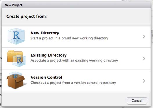
These options let you decide from where you want to create your project. So, if you want to start it from scratch and create a new directory, associate your new project to an existing one, or if you want to create a project from a version control repository, you can avail of the respective options. For now, we will focus on creating a new directory.
The following list will show you the next options available:
- Empty Project
- R Package
- Shiny Web Application
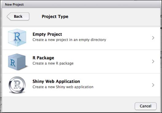
We will look in the categories, R Package and Shiny Web Application later in this book, so for now we will concentrate on the Empty Project option.
A very important question you have to ask yourself when creating a new project is where you want to save it? There are several options and details you have to pay attention to especially when it comes to collaboration and different people working on the same project.
You can save your project locally, on a cloud storage or with the help of a revision control system such as Git.
An easy way to store your project and to be able to access it from everywhere is the use of a cloud storage provider like Dropbox. It offers you a free account with 2 GB of storage, which should be enough for your first project.
RStudio actively monitors your project files for changes, which allows it to index functions and files to enable code completion and navigation. But when you use Dropbox at the same time to remotely sync your work, it will also monitor your files and this can cause conflicts. So you should tell Dropbox to ignore the .Rproj.user directory in your RStudio project.
To ignore a file in Dropbox, navigate to Preferences | Account | Selective Sync and uncheck the .Rproj.user directory.
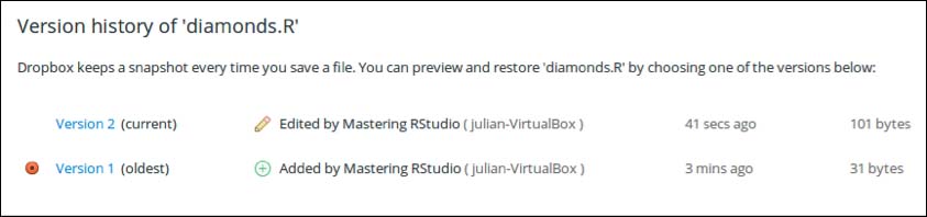
Dropbox also helps you with version control, as it keeps previous versions of a file.
To begin your first project, choose the New Directory option we described before and create an empty project. Then, choose a name for the directory and the location that you want to save it in. You should create a projects folder on your Dropbox.
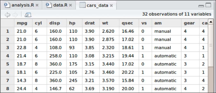
The first project will be a small data analysis based on a dataset that was extracted from the 1974 issue of the Motor Trend US magazine. It comprises fuel consumption and ten aspects of automobile design and performance, such as the weight or number of cylinders for 32 automobiles, and is included in the base R package. So, we do not have to install a separate package to work with this dataset, as it is automatically loaded when you start R.
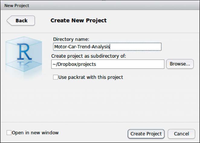
As you can see, we left the Use packrat with this project option unchecked. Packrat is a dependency management tool that makes your R code more isolated, portable, and reproducible by giving your project its own privately managed package library. This is especially important when you want to create projects in an organizational context where the code has to run on various computer systems, and has to be usable for a lot of different users. This first project will just run locally and will not focus on a specific combination of package versions.
RStudio creates an empty directory for you that includes just the file, Motor-Car-Trend-Analysis.Rproj. This file will store all the information on your project that RStudio will need for loading. But to stay organized, we have to create some folders in the directory. Create the following folders:
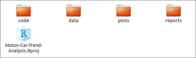
This is a very basic folder structure and you have to adapt it to your needs in your own projects. You could, for example, add the folders, raw and processed, in the data folder. Raw for unstructured data that you started with, and processed for cleaned data that you actually used for your analysis.
The Motor Trend Car Road Tests dataset is part of the dataset package, which is one of the preinstalled packages in R. But, we will save the data in a CSV file in our data folder, after extracting the data from the mtcars variable, to make sure our analysis is reproducible:
#write data into csv file
write.csv(mtcars, file = "data/cars.csv", row.names=FALSE)
Put the previous line of code in a new R script and save it as data.R in the code folder.
The analysis script will first have to load the data from the CSV file with the following line:
cars_data <- read.csv(file = "data/cars.csv", header = TRUE, sep = ",")
If you want to create a report from your R script, you have to specify the relative path to the data file, beginning with two dots:
cars_data <- read.csv(file = "../data/cars.csv", header = TRUE, sep = ",")
Next, we can take a look at the different variables and see if we can find any correlations on the first look. We can create a pairs matrix with the following line:
pairs(cars_data)
We can then save the created matrix with the export function of the Plots Pane option. Then, we can save it as an image in the plots folder:
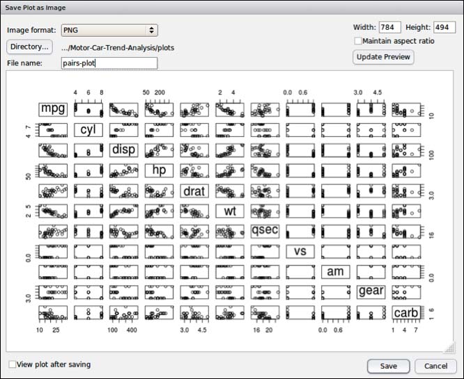
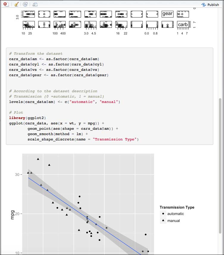
As you can see, we can expect a lot of different variable combinations, which could correlate very well. The most obvious one is surely weight of the car (wt) and Miles per Gallon (mpg): a heavy car seems to need more gallons of fuel than a lighter car.
We can now test this hypothesis by calculating the correlation and plotting a scatterplot of these two variables. In addition, we can also do a linear regression and see how it performs:
cor(cars_data$wt, cars_data$mpg)


install.packages("ggplot2")
require(ggplot2)

ggplot(cars_data, aes(x=wt, y=mpg))+
  geom_point(aes(shape=factor(am, labels = c("Manual","Automatic"))))+
  geom_smooth(method=lm)+scale_shape_discrete(name = "Transmission Type")

firstModel <- lm(mpg~wt, data = cars_data)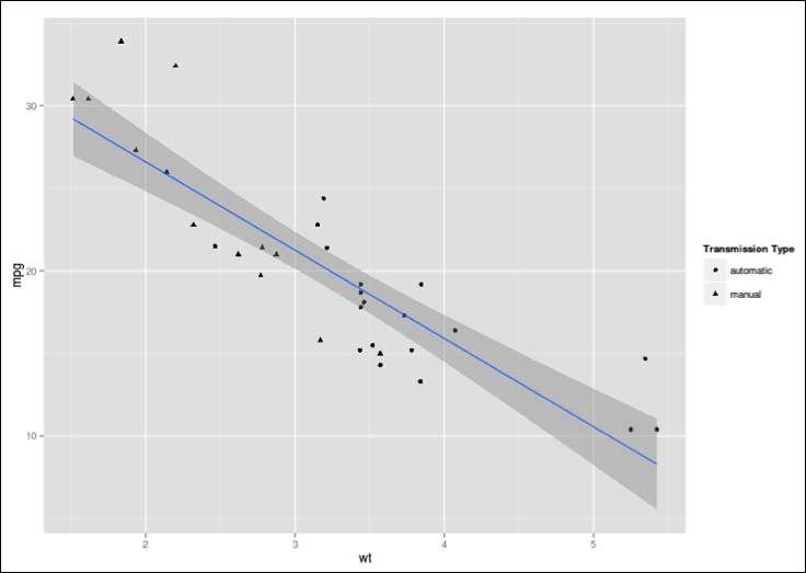
We can see more details with:
summary(firstModel)$coef

[1] -0.8676594

print(c('R-squared', round(summary(firstModel)$r.sq,2)))

[1] "R-squared"  "0.75"
We can see that there is a high negative correlation between these two variables, and the first model is a pretty good fit with an R-squared value of 0.75.
But we also have to test other combinations and see how they perform. And what we basically do is test all the correlations and use the best model.
We will not explain the statistical functions behind this approach, as it would be out of the scope of this chapter:
#Test other correlations
completeModel <- lm(mpg ~., data=cars_data)
stepSolution <- step(completeModel, direction = "backward")

#get the best model
bestModel <- stepSolution$call
bestModel
The output will look like this:
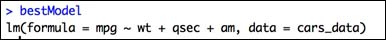
The best model now has the following formula:
mpg ~ wt + qsec + am
So, we will create a final model with this formula and see how it performs:
finalModel <- lm(mpg~wt + factor(am) + qsec, data = cars_data)
summary(finalModel)$coef
print(c('R-squared', round(summary(finalModel)$r.sq,2)))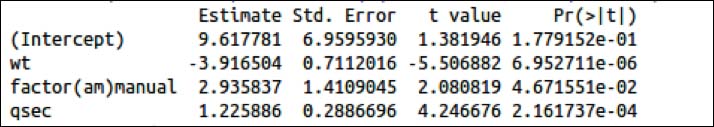
[1] "R-squared" "0.85"
As we can see, the final model also includes the variable, qsec, which is the time the car needs for a quarter mile, and am, which is the type of transmission (automatic or manual).
But, we can also see that just the transmission type, manual, seems to play a significant role when it comes to mileage.
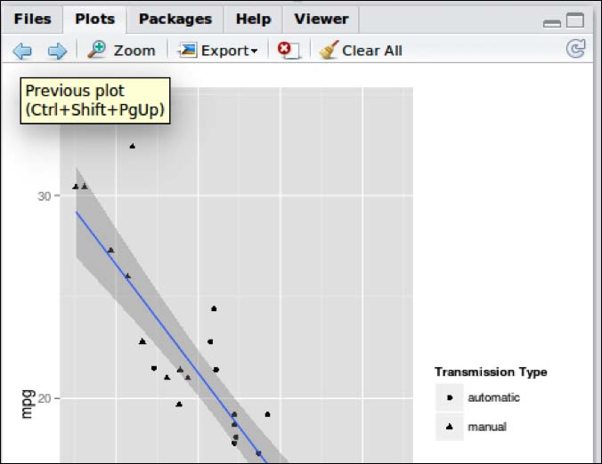
After you execute the analysis script, you can see that all your results are still in RStudio, which is a big advantage in contrast to the R console.
So, you can go through all the graphs you produced in the plot viewer with the arrows.
Or, you can see which variables are set in the environment. These are all the models you calculated in this analysis, as well as in your initial dataset.
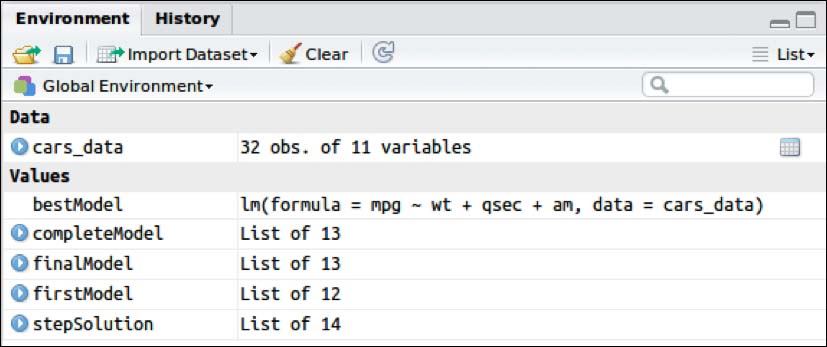
You can click on the table icon behind cars_data in the Environment pane to open the data frame in the Source pane.