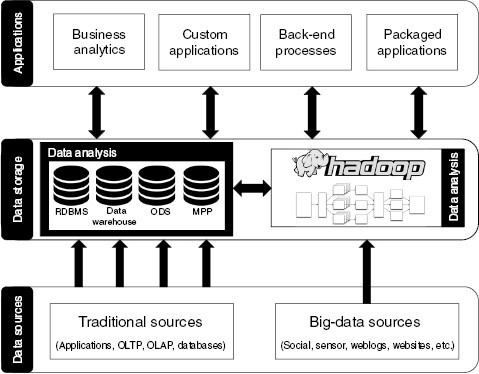
Figure 6 A typical small-data and big-data architecture for data science (inspired by a figure from the Hortonworks newsletter, April 23, 2013, https://hortonworks.com/blog/hadoop-and-the-data-warehouse-when-to-use-which).
The set of technologies used to do data science varies across organizations. The larger the organization or the greater the amount of data being processed or both, the greater the complexity of the technology ecosystem supporting the data science activities. In most cases, this ecosystem contains tools and components from a number of different software suppliers, processing data in many different formats. There is a spectrum of approaches from which an organization can select when developing its own data science ecosystem. At one end of the spectrum, the organization may decide to invest in a commercial integrated tool set. At the other end, it might build up a bespoke ecosystem by integrating a set of open-source tools and languages. In between these two extremes, some software suppliers provide solutions that consist of a mixture of commercial products and open-source products. However, although the particular mix of tools will vary from one organization to the next, there is a commonality in terms of the components that are present in most data science architectures.
Figure 6 gives a high-level overview of a typical data architecture. This architecture is not just for big-data environments, but for data environments of all sizes. In this diagram, the three main areas consist of data sources, where all the data in an organization are generated; data storage, where the data are stored and processed; and applications, where the data are shared with consumers of these data.
Figure 6 A typical small-data and big-data architecture for data science (inspired by a figure from the Hortonworks newsletter, April 23, 2013, https://hortonworks.com/blog/hadoop-and-the-data-warehouse-when-to-use-which).
All organizations have applications that generate and capture data about customers, transactions, and operational data on everything to do with how the organization operates. Such data sources and applications include customer management, orders, manufacturing, delivery, invoicing, banking, finance, customer-relationship management (CRM), call center, enterprise resource planning (ERP) applications, and so on. These types of applications are commonly referred to as online transaction processing (OLTP) systems. For many data science projects, the data from these applications will be used to form the initial input data set for the ML algorithms. Over time, the volume of data captured by the various applications in the organization grows ever larger and the organization will start to branch out to capture data that was ignored, wasn’t captured previously, or wasn’t available previously. These newer data are commonly referred to as “big-data sources” because the volume of data that is captured is significantly higher than the organization’s main operational applications. Some of the common big-data sources include network traffic, logging data from various applications, sensor data, weblog data, social media data, website data, and so on. In traditional data sources, the data are typically stored in a database. However, because the applications associated with many of the newer big-data sources are not primarily designed to store data long term—for example, with streaming data—the storage formats and structures for this type of data vary from application to application.
As the number of data sources increases, so does the challenge of being able to use these data for analytics and for sharing them across the wider organization. The data-storage layer, shown in figure 6, is typically used to address the data sharing and data analytics across an organization. This layer is divided into two parts. The first part covers the typical data-sharing software used by most organizations. The most popular form of traditional data-integration and storage software is a relational database management system (RDBMS). These traditional systems are often the backbone of the business intelligence (BI) solutions within an organization. A BI solution is a user-friendly decision-support system that provides data aggregating, integration, and reporting as well as analysis functionality. Depending on the maturity level of a BI architecture, it can consist of anything from a basic copy of an operational application to an operational data store (ODS) to massively parallel processing (MPP) BI database solutions and data warehouses.
Data warehousing is best understood as a process of data aggregation and analysis with the goal of supporting decision making. However, the focus of this process is the creation of a well-designed and centralized data repository, and the term data warehouse is sometimes used to denote this type of data repository. In this sense, a data warehouse is a powerful resource for data science. From a data science perspective, one of the major advantages of having a data warehouse in place is a much shorter project time. The key ingredient in any data science process is data, so it is not surprising that in many data science projects the majority of time and effort goes into finding, aggregating, and cleaning the data prior to their analysis. If a data warehouse is available in a company, then the effort and time that go into data preparation on individual data science projects is often significantly reduced. However, it is possible to do data science without a centralized data repository. Constructing a centralized repository of data involves more than simply dumping the data from multiple operational databases into a single database.
Merging data from multiple databases often requires much complex manual work to resolve inconsistencies between the source databases. Extraction, transformation, and load (ETL) is the term used to describe the typical processes and tools used to support the mapping, merging, and movement of data between databases. The typical operations carried out in a data warehouse are different from the simple operations normally applied to a standard relational data model database. The term online analytical processing (OLAP) is used to describe these operations. OLAP operations are generally focused on generating summaries of historic data and involve aggregating data from multiple sources. For example, we might pose the following OLAP request (expressed here in English for readability): “Report the sales of all stores by region and by quarter and compare these figures to last year’s figures.” What this example illustrates is that the result of an OLAP request often resembles what you would expect to see as a standard business report. OLAP operations essentially enable users to slice, dice, and pivot the data in the warehouse and get different views of these data. They work on a data representation called a data cube that is built on top of the data warehouse. A data cube has a fixed, predefined set of dimensions in which each dimension represents a particular characteristic of the data. The required data-cube dimensions for the example OLAP request given earlier would be sales by stores, sales by region, and sales by quarter. The primary advantage of using a data cube with a fixed set of dimensions is that it speeds up the response time of OLAP operations. Also, because the set of data-cube dimensions is preprogrammed into the OLAP system, the system can provide user-friendly graphical user interfaces for defining OLAP requests. However, the data-cube representation also restricts the types of analysis that can be done using OLAP to the set of queries that can be generated using the predefined dimensions. By comparison, SQL provides a more flexible query interface. Also, although OLAP systems are useful for data exploration and reporting, they don’t enable data modeling or the automatic extraction of patterns from the data. Once the data from across an organization has been aggregated and analyzed within the BI system, this analysis can then be used as input to a range of consumers in the applications layer of figure 6.
The second part of the data-storage layer deals with managing the data produced by an organization’s big-data sources. In this architecture, the Hadoop platform is used for the storage and analytics of these big data. Hadoop is an open-source framework developed by the Apache Software Foundation that is designed for the processing of big data. It uses distributed storage and processing across clusters of commodity servers. Applying the MapReduce programming model, it speeds up the processing of queries on large data sets. MapReduce implements the split-apply-combine strategy: (a) a large data set is split up into separate chunks, and each chunk is stored on a different node in the cluster; (b) a query is then applied to all the chunks in parallel; and (c) the result of the query is then calculated by combining the results generated on the different chunks. Over the past couple of years, however, the Hadoop platform is also being used as an extension of an enterprise’s data warehouse. Data warehouses originally would store three years of data, but now data warehouses can store more than 10 years of data, and this number keeps increasing. As the amount of data in a data warehouse increases, however, the storage and processing requirements of the database and server also have to increase. This requirement can have a significant cost implication. An alternative is to move some of the older data in a data warehouse for storage into a Hadoop cluster. For example, the data warehouse would store the most recent data, say three years’ worth of data, which frequently need to be available for quick analysis and presentation, while the older data and the less frequently used data are stored on Hadoop. Most of the enterprise-level databases have features that connect the data warehouse with Hadoop, allowing a data scientist, using SQL, to query the data in both places as if they all are located in one environment. Her query could involve accessing some data in the data-warehouse database and some of the data in Hadoop. The query processing will be automatically divided into two distinct parts, each running independently, and the results will be automatically combined and integrated before being presented back to the data scientist.
Data analysis is associated with both sections of the data-storage layer in figure 6. Data analysis can occur on the data in each section of the data layer, and the results from data analysis can be shared between each section while additional data analysis is being performed. The data from traditional sources frequently are relatively clean and information dense compared to the data captured from big-data sources. However, the volume and real-time nature of many big-data sources means that the effort involved in preparing and analyzing these big-data sources can be repaid in terms of additional insights not available through the data coming from traditional sources. A variety of data-analysis techniques developed across a number of different fields of research (including natural-language processing, computer vision, and ML) can be used to transform unstructured, low-density, low-value big data into high-density and high-value data. These high-value data can then be integrated with the other high-value data from traditional sources for further data analysis. The description given in this chapter and illustrated in figure 6 is the typical architecture of the data science ecosystem. It is suitable for most organizations, both small and large. However, as an organization scales in size, so too will the complexity of its data science ecosystem. For example, smaller-scale organizations may not require the Hadoop component, but for very large organizations the Hadoop component will become very important.
The traditional approach to data analysis involves the extraction of data from various databases, integrating the data, cleaning the data, subsetting the data, and building predictive models. Once the prediction models have been created they can be applied to the new data. Recall from chapter 1 that a prediction model predicts the missing value of an attribute: a spam filter is a prediction model that predicts whether the classification attribute of an email should have the value of “spam” or not. Applying the predictive models to the instances in new data to generate the missing values is known as “scoring the data.” Then the final results, after scoring new data, may be loaded back into a database so that these new data can be used as part of some workflow, reporting dashboard, or some other company assessment practice. Figure 7 illustrates that much of the data processing involved in data preparation and analysis is located on a server that is separate from the databases and the data warehouse. Therefore, a significant amount of time can be spent just moving the data out of the database and moving the results back into the database.
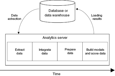
Figure 7 The traditional process for building predictive models and scoring data.
An experiment run at the Dublin Institute of Technology on building a linear-regression model supplies an example of the time involved in each part of the process. Approximately 70 to 80 percent of the time is taken with extracting and preparing the data; the remaining time is spent on building the models. For scoring data, approximately 90 percent of the time is taken with extracting the data and saving the scored data set back into the database; only 10 percent of the time is spent on actually scoring. These results are based on data sets consisting of anywhere from 50,000 records up to 1.5 million records. Most enterprise database vendors have recognized the time savings that would be available if time did not have to be spent on moving data and have responded to this problem by incorporating data-analysis functionality and ML algorithms into their database engines. The following sections explore how ML algorithms have been integrated into modern databases, how data storage works in the big-data world of Hadoop, and how using a combination of these two approaches allows organizations to easily work with all their data using SQL as a common language for accessing, analyzing, and performing ML and predictive analytics in real time.
Database vendors continuously invest in developing the scalability, performance, security, and functionality of their databases. Modern databases are far more advanced than traditional relational databases. They can store and query data in variety of different formats. In addition to the traditional relational formats, it is also possible to define object types, store documents, and store and query JSON objects, spatial data, and so on. Most modern databases also come with a large number of statistical functions, so that some have an equivalent number of statistical functions as most statistical applications. For example, the Oracle Database comes with more than 300 different statistical functions and the SQL language built into it. These statistical functions cover the majority of the statistical analyses needed by data science projects and include most if not all the statistical functions available in other tools and languages, such as R. Using the statistical functionality that is available in the databases in an organization may allow data analytics to be performed in a more efficient and scalable manner using SQL. Furthermore, most leading database vendors (including Oracle, Microsoft, IBM, and EnterpriseDB) have integrated many ML algorithms into their databases, and these algorithms can be run using SQL. ML that is built into the database engine and is accessible using SQL is known as in-database machine learning. In-database ML can lead to quicker development of models and quicker deployment of models and results to applications and analytic dashboards. The idea behind the in-database ML algorithms is captured in the following directive: “Move the algorithms to the data instead of the data to the algorithms.”
The main advantages of using the in-database ML algorithms are:
Many organizations are exploiting the benefits of in-database ML. They range from small and medium organizations to large, big-data-type organizations. Some examples of organizations that use in-database ML technologies are:
Although the traditional (modern) database is incredibly efficient at processing transactional data, in the age of big data new infrastructure is required to manage all the other forms of data and for longer-term storage of the data. The modern traditional database can cope with data volumes up to a few petabytes, but for this scale of data, traditional database solutions may become prohibitively expensive. This cost issue is commonly referred to as vertical scaling. In the traditional data paradigm, the more data an organization has to store and process within a reasonable amount of time, the larger the database server required and in turn the greater the cost for server configuration and database licensing. Organizations may be able to ingest and query one billion records on a daily/weekly bases using traditional databases, but for this scale of processing they may need to invest more than $100,000 just purchasing the required hardware.
Hadoop is an open-source platform developed and released by the Apache Software Foundation. It is a well-proven platform for ingesting and storing large volumes of data in an efficient manner and can be much less expensive than the traditional database approach. In Hadoop, the data are divided up and partitioned in a variety of ways, and these partitions or portions of data are spread across the nodes of the Hadoop cluster. The various analytic tools that work with Hadoop process the data that reside on each of the nodes (in some instances these data can be memory resident), thus allowing for speedy processing of the data because the analytics is performed in parallel across the nodes. No data extraction or ETL process is needed. The data are analyzed where they are stored.
Although Hadoop is the best known big-data processing framework, it is by no means the only one. Other big-data processing frameworks include Storm, Spark, and Flink. All of these frameworks are part of the Apache software foundation projects. The difference between these frameworks lies in the fact that Hadoop is primarily designed for batch processing of data. Batch processing is appropriate where the dataset is static during the processing and where the results of the processing are not required immediately (or at least are not particularly time sensitive). The Storm framework is designed for processing streams of data. In stream processing each element in the stream is processed as it enters the system, and consequently the processing operations are defined to work on each individual element in the stream rather than on the entire data set. For example, where a batch process might return an average over a data set of values, a stream process will return an individual label or value for each element in the stream (such as calculating a sentiment score for each tweet in a Twitter stream). Storm is designed for real-time processing of data and according to the Storm website,1 it has been benchmarked at processing over a million tuples per second per node. Spark and Flink are both hybrid (batch and stream) processing frameworks. Spark is a fundamentally a batch processing framework, similar to Hadoop, but also has some stream processing capabilities whereas Flink is a stream processing framework that can also be used for batch processing. Although these big-data processing frameworks provide data scientists with a choice of tools to meet the specific big-data requirements of their project using these frameworks can have the drawback that the modern data scientist now has to analyze data in two different locations, in the traditional modern databases and in the big-data storage. The next section looks at how this particular issue is being addressed.
If an organization does not have data of the size and scale that require a Hadoop solution, then it will require only traditional database software to manage its data. However, some of the literature argues that the data-storage and processing tools available in the Hadoop world will replace the more traditional databases. It is very difficult to see this happening, and more recently there has been much discussion about having a more balanced approach to managing data in what is called the “hybrid database world.” The hybrid database world is where traditional databases and the Hadoop world coexist.
In the hybrid database world, the organization’s databases and Hadoop-stored data are connected and work together, allowing the efficient processing, sharing, and analysis of the data. Figure 8 shows a traditional data warehouse, but instead of all the data being stored in the database or the data warehouse, the majority of the data is moved to Hadoop. A connection is created between the database and Hadoop, which allows the data scientist to query the data as if they all are in one location. The data scientist does not need to query the portion of data that is in the database warehouse and then in a separate step query the portion that is stored in Hadoop. He can query the data as he always has done, and the solution will identify what parts of the query need to be run in each location. The results of the query arrived at in each location will be merged together and presented to him. Similarly, as the data warehouse grows, some the older data will not be queried as frequently. The hybrid database solution automatically moves the less frequently used data to the Hadoop environment and the more frequently used data to the warehouse. The hybrid database automatically balances the location of the data based on the frequency of access and the type of data science being performed.
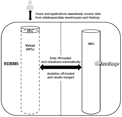
Figure 8 Databases, data warehousing, and Hadoop working together (inspired by a figure in the Gluent data platform white paper, 2017, https://gluent.com/wp-content/uploads/2017/09/Gluent-Overview.pdf).
One of the advantages of this hybrid solution is that the data scientist still uses SQL to query the data. He does not have to learn another data-query language or have to use a variety of different tools. Based on current trends, the main database vendors, data-integration solution vendors, and all cloud data-storage vendors will have solutions similar to this hybrid one in the near future.
Data integration involves taking the data from different data sources and merging them to give a unified view of the data from across the organization. A good example of such integration occurs with medical records. Ideally, every person would have one health record, and every hospital, medical facility, and general practice would use the same patient identifier or same units of measures, the same grading system, and so on. Unfortunately, nearly every hospital has its own independent patient-management system, as does each of the medical labs within the hospital. Think of the challenges in finding a patient’s record and assigning the correct results to the correct patient. And these are the challenges faced by just one hospital. In scenarios where multiple hospitals share patient data, the problem of integration becomes significant. It is because of these kind of challenges that the first three CRISP-DM stages take up to 70 to 80 percent of the total data science project time, with the majority of this time being allocated to data integration.
Integrating data from multiple data sources is difficult even when the data are structured. However, when some of the newer big-data sources are involved, where semi- or unstructured data are the norm, then the cost of integrating the data and managing the architecture can become significant. An illustrative example of the challenges of data integration is customer data. Customer data can reside in many different applications (and the applications’ corresponding databases). Each application will contain a slightly different piece of customer data. For example, the internal data sources might contain the customer credit rating, customer sales, payments, call-center contact information, and so on. Additional data about the customer may also be available from external data sources. In this context, creating an integrated view of a customer requires the data from each of these sources to be extracted and integrated.
The typical data-integration process will involve a number of different stages, consisting of extracting, cleaning, standardizing, transforming, and finally integrating to create a single unified version of the data. Extracting data from multiple data sources can be challenging because many data sources can be accessed only by using an interface particular to that data source. As a consequence, data scientists need to have a broad skill set to be able to interact with each of the data sources in order to obtain the data.
Once data have been extracted from a data source, the quality of the data needs to be checked. Data cleaning is a process that detects, cleans, or removes corrupt or inaccurate data from the extracted data. For example, customer address information may have to be cleaned in order to convert it into a standardized format. In addition, there may be duplicate data in the data sources, in which case it is necessary to identify the correct customer record that should be used and to remove all the other records from the data sets. It is important to ensure that the values used in a data set are consistent. For example, one source application might use numeric values to represent a customer credit rating, but another might have a mixture of numeric and character values. In such a scenario, a decision regarding what value to use is needed, and then the other representations should be mapped into the standardized representation. For example, imagine one of the attributes in the data set is a customer’s shoe size. Customers can buy shoes from various regions around the world, but the numbering system used for shoe sizes in Europe, the United States, the United Kingdom, and other countries are slightly different. Prior to doing data analysis and modeling, these data values need to be standardized.
Data transformation involves the changing or combining of the data from one value to another. A wide variety of techniques can be used during this step and include data smoothing, binning, and normalization as well as writing custom code to perform a particular transformation. A common example of data transformation is with processing a customer’s age. In many data science tasks, precisely distinguishing between customer ages is not particularly helpful. The difference between a 42-year-old customer and a 43-year-old customer is generally not significant, although differentiating between a 42-year-old customer and a 52-year-old customer may be informative. As a consequence, a customer’s age is often transformed from a raw age into a general age range. This process of converting ages into age ranges is an example of a data-transformation technique called binning. Although binning is relatively straightforward from a technical perspective, the challenge here is to identify the most appropriate range thresholds to apply during binning. Applying the wrong thresholds may obscure important distinctions in the data. Finding appropriate thresholds, however, may require domain specific knowledge or a process of trial-and-error experimentation.
The final step in data integration involves creating the data that are used as input to the ML algorithms. This data is known as the analytics base table.
The most important step in creating the analytics base table is the selection of the attributes that will be included in the analysis. The selection is based on domain knowledge and on an analysis of the relationships between attributes. Consider, for example, a scenario where the analysis is focused on customers of a service. In this scenario, some of the frequently used domain concepts that will inform the design and selection of attributes include customer contract details, demographics, usage, changes in usage, special usage, life-cycle phase, network links, and so on. Furthermore, attributes that are found to have a high correlation with other attributes are likely to be redundant, and so one of the correlated attributes should be excluded. Removing redundant features can result in simpler models which are easier to understand, and also reduces the likelihood of an ML algorithm returning a model that is fitted to spurious patterns in the data. The set of attributes selected for inclusion define what is known as the analytics record. An analytics record typically includes both raw and derived attributes. Each instance in the analytics base table is represented by one analytics record, so the set of attributes included in the analytics record defines the representation of the instances the analysis will be carried out on.
After the analytics record has been designed, a set of records needs to extracted and aggregated to create a data set for analysis. When these records have been created and stored—for example, in a database—this data set is commonly referred to as the analytics base table. The analytics base table is the data set that is used as input to the ML algorithms. The next chapter introduces the field of ML and describes some of the most popular ML algorithms used in data science.