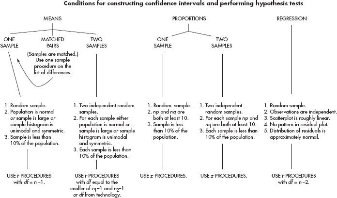
CHECKING ASSUMPTIONS FOR INFERENCE
THE TOP TEN
1. Graders want to give you credit—help them! Make them understand what you are doing, why you are doing it, and how you are doing it. Don’t make the reader guess at what you are doing. Communication is just as important as statistical knowledge!
2. For both multiple-choice and free-response questions, read the question carefully! Be sure you understand exactly what you are being asked to do or find or explain.
3. Check assumptions. Don’t just state them! Be sure the assumptions to be checked are stated correctly. Verifying assumptions and conditions means more than simply listing them with little check marks—you must show work or give some reason to confirm verification.
4. Learn and practice how to read generic computer output. And in answering questions using computer output, realize that you usually will not need to use all the information given.
5. Naked or bald answers will receive little or no credit! You must show where answers come from. On the other hand, don’t give more than one solution to the same problem—you will receive credit only for the weaker one.
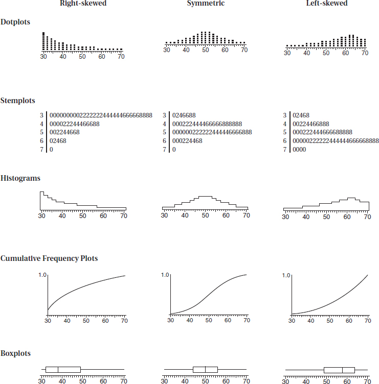
6. If you refer to a graph, whether it is a histogram, boxplot, stemplot, scatterplot, residuals plot, normal probability plot, or some other kind of graph, you should roughly draw it. It is not enough to simply say, “I did a normal probability plot of the residuals on my calculator and it looked linear.” Be sure to label axes and show number scales whenever possible.
7. Use proper terminology! For example, the language of experiments is different from the language of observational studies—you shouldn’t mix up blocking and stratification. Know what confounding means and when it is proper to use this term. Replication on many subjects to reduce chance variation is different from replication of an experiment itself to achieve validation.
8. Avoid “calculator speak”! For example, do not simply write “2-SampTTest …” or “binomcdf…” There are lots of calculators out there, each with its own abbreviations. Some abbreviated function notation can be referenced IF the parameters used are identified.
9. Be careful about using abbreviations in general. For example, your teacher might use LOBF (line of best fit), but the grader may have no idea what this refers to.
10. Don’t automatically “parrot” the stem of the problem! For example, the question might refer to sample data; however, your hypotheses must be stated in terms of a population parameter.
25 MORE HINTS
11. Insert new calculator batteries or carry replacement batteries with you.
12. Underline key words and phrases while reading questions.
13. Some problems look scary on first reading but are not overly difficult and are surprisingly straightforward if you approach them systematically. And some questions might take you beyond the scope of the AP curriculum; however, remember that they will be phrased in such ways that you should be able to answer them based on what you have learned in your AP Stat class.
14. Read through all six free-response questions, underlining key points. Go back and do those questions you think are easiest (this will usually, but not always, include Problem 1). Then tackle the heavily weighted Problem 6 for a while. Finally, try the remaining problems. If you have a few minutes at the end to try some more on Problem 6, that’s great!
15. Answers do not have to be in paragraph form. Symbols and algebra are fine. Just be sure that your method, reasoning, and calculations will be clear to the reader, and that the explanations and conclusions are given in context of the problem.
16. If you show calculations carefully, a wrong answer due to a computational error might still result in full credit.
17. If you can’t solve part of a problem, but that solution is necessary to proceed, make up a reasonable answer to the first part and use this to proceed to the remaining parts of the problem.
18. When using a formula, write down the formula and then substitute the values.
19. Conclusions should be stated in proper English. For example, don’t use double negatives.
20. Read carefully and recognize that sometimes very different tests are required in different parts of the same problem.
21. Realize that there may be several reasonable approaches to a given problem. In such cases pick either the one you feel most comfortable with or the one you feel will require the least time.
22. Realize that there may not be one clear, correct answer. Some questions are designed to give you an opportunity to creatively synthesize a relationship among the problem’s statistical components.
23. Punching a long list of data into the calculator doesn’t show statistical knowledge. Be sure it’s necessary!
24. Remember that uniform and symmetric are not the same, and that not all symmetric unimodal distributions are normal.
25. When making predictions and interpreting slopes and intercepts, don’t become confused between your original data and your regression model.
26. If the slope is close to ±1, it does not follow that the correlation is strong.
27. When describing residual graphs, “randomly scattered” does not mean the same as “half below and half above.” You should comment on whether or not there are nonlinear patterns, and increasing or decreasing spread, and on whether the residuals are small or large compared to the associated y-values.
28. Simply using a calculator to find a regression line is not enough; you must understand it (for example, be able to interpret the slope and intercepts in context).
29. With regard to hypothesis test problems, (1) the hypotheses must be stated in terms of population parameters with all variables clearly defined; (2) the test must be specified by name or formula, and you must show how the test assumptions are met; (3) the test statistic and associated P-value should be calculated; (4) the P-value must be linked to a decision; and (5) a conclusion must be stated in the context of the problem.
30. For any inference problem, be sure to ask yourself whether the variable is categorical (usually leading to proportions) or quantitative (usually leading to means), whether you are working with raw data or summary statistics, whether there is a single population of interest or two populations being compared, and in the case of comparison whether there are independent samples or a paired comparison.
31. A simple random sample (SRS) and a random assignment of treatments to subjects both have to do with randomness, but they are not the same. Understand the difference!
32. Simply saying to “randomly assign” subjects to treatment groups is usually an incomplete response. You need to explain how to make the assignments, for example, using a random number table or through generating random numbers on a calculator.
33. Blinding and placebos in experiments are important but are not always feasible. You can still have “experiments” without these.
34. The distribution of a particular sample (data set) is not the same as the sampling distribution of a statistic. Understand the difference!
35. Just because a sample is large does not imply that the distribution of the sample will be close to a normal distribution.
The Multiple-Choice and Free-Response sections are weighted equally.
There is no penalty for guessing in the Multiple-Choice section.
The Investigative Task counts for 25% of the Free-Response section. Each of the Free-Response questions has a possible four points.
To find your score use the following guide:
Multiple-Choice section (40 questions)
Number correct × 1.25 = __________
Free-Response section (5 Open-Ended questions plus an Investigative Task)
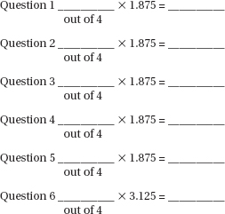
Total points from Multiple-Choice and Free-Response sections = __________
Conversion chart based on a recent AP exam
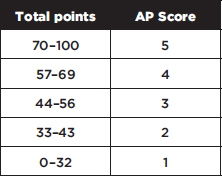
In the past, roughly 10% of students scored 5, 20% scored 4, 25% scored 3, 20% scored 2, and 25% scored 1 on the AP Statistics exam. Colleges generally require a score of at least 3 for a student to receive college credit.
There are many more useful features than introduced below—see the guidebook that comes with the calculator. For reference, following is a listing of the basic uses with which all students should be familiar. However, always remember that the calculator is only a tool, that it will find minimal use in the multiple-choice section, and that “calculator talk” (calculator syntax) should NOT be used in the free-response section.
Plotting statistical data:
STAT PLOT allows one to show scatterplots, histograms, modified boxplots, and regular boxplots of data stored in lists. Note the use of TRACE with the various plots.
Numerical statistical data:
1-Var Stats gives the mean, standard deviation, and 5-number summary of a list of data.
Binomial probabilities:
binompdf (n, p, x) gives the probability of exactly x successes in n trials where p is the probability of success on a single trial.
binomcdf (n, p, x) gives the cumulative probability of x or fewer successes in n trials where p is the probability of success on a single trial.
Geometric probabilities:
geometpdf (p, x) gives the probability that the first success occurs on the x-th trial, where p is the probability of success on a single trial.
geometcdf (p, x) gives the cumulative probability that the first success occurs on or before the x-th trial, where p is the probability of success on a single trial.
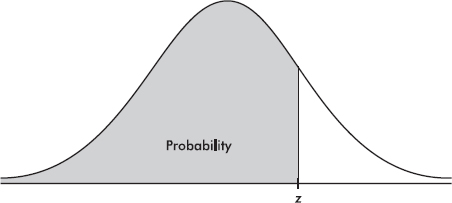
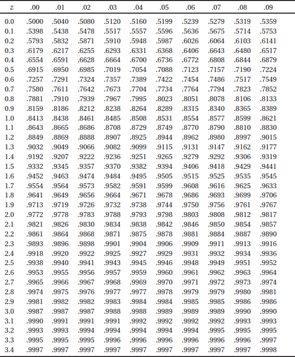
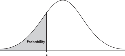
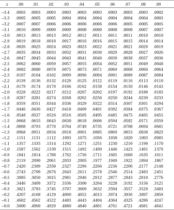
The normal distribution:
normalcdf (lowerbound, upperbound, µ,  ) gives the probability that a score is between the two bounds for the designated mean µ and standard deviation . The defaults are µ = 0 and = 1.
InvNorm (area, µ, ) gives the score associated with an area (probability) to the left of the score for the designated mean µ and standard deviation . The defaults are µ = 0 and = 1.
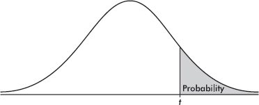
The t-distribution:
tcdf (lowerbound, upperbound, df) gives the probability a score is between the two bounds for the specified df (degrees of freedom).
invT(area, df) gives the t-score associated with an area (probability) to the left of the score under the student t-probability function for the specified df (degrees of freedom). [Note: this is available on the new operating system for the TI-84+.]
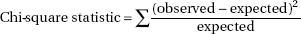
The chi-square distribution:
 2cdf (lowerbound, upperbound, df) gives the probability a score is between the two bounds for the specified df (degrees of freedom).
2GOF-Test is a chi-square goodness-of-fit test to confirm whether sample data conforms to a specified distribution. [Note: this is available on the new operating system for the TI-84+.]
Linear regression and correlation:
LinReg (ax + b) fits the equation y = ax + b to the data in lists L1 and L2 using a least-squares fit. When DiagnosticOn is set, the values for r2 and r are also displayed.
Confidence intervals:
For proportions—
1-PropZInt gives a confidence interval for a proportion of successes.
2-PropZInt gives a confidence interval for the difference between the proportion of successes in two populations.
For means—
TInterval gives a confidence interval for a population mean (use the t-distribution because population variances are never really known).
2-SampTInt gives a confidence interval for the difference between two population means.
Hypothesis tests:
For proportions—
1-PropZTest
2-PropZTest compares the proportion of successes from two populations (making use of the pooled sample proportion).
For means—
T-Test
2-SampTTest
For chi-square test for association—
2-Test gives the 2-value and P-value for the null hypothesis H0: no association between row and column variables, and the alternative hypothesis Ha: the variables are related. The observed counts must first be entered into a matrix.
For linear regression—
LinRegTTest calculates a linear regression and performs a t-test on the null hypothesis H0:  = 0 (H0: ρ = 0). The regression equation is stored in RegEQ (under VARS Statistics EQ) and the list of residuals is stored in RESID (under LIST NAMES).
Catalog help:
To activate Catalog Help, press APPS, choose CtlgHelp, and press ENTER. Then, for example, if you press 2nd, DISTR, arrow down to normalcdf, and press +, you are prompted to insert (lowerbound, upperbound, [µ,]), that is, to insert the bounds and, optionally, the mean and SD.
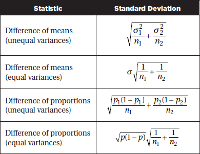
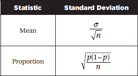
The following are in the form and notation as recommended by the College Board.
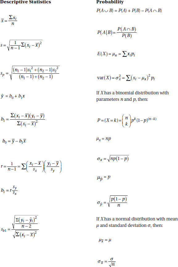

Confidence interval:
Estimate ± (critical value) · (standard deviation of the estimate)
SINGLE SAMPLE
TWO SAMPLE