
I am going to divide this lecture into two parts. First, I am going to talk about problems associated with the theory of quantum electrodynamics itself, supposing that all there is in the world is electrons and photons. Then I will talk about the relation of quantum electrodynamics to the rest of physics.
The most shocking characteristic of the theory of quantum electrodynamics is the crazy framework of amplitudes, which you might think indicates problems of some sort! However, physicists have been fiddling around with amplitudes for more than fifty years now, and have gotten very used to it. Furthermore, all the new particles and new phenomena that we are able to observe fit perfectly with everything that can be deduced from such a framework of amplitudes, in which the probability of an event is the square of a final arrow whose length is determined by combining arrows in funny ways (with interferences, and so on). So this framework of amplitudes has no experimental doubt about it: you can have all the philosophical worries you want as to what the amplitudes mean (if, indeed, they mean anything at all), but because physics is an experimental science and the framework agrees with experiment, it’s good enough for us so far.
There is a set of problems associated with the theory of quantum electrodynamics that has to do with improving the method of calculating the sum of all the little arrows—various techniques that are available in different circumstances—that take the graduate students three or four years to master. Since they are technical problems, I am not going to discuss them here. It’s just a matter of continuously improving the techniques for analyzing what the theory really has to say in different circumstances.
But there is one additional problem that is characteristic of the theory of quantum electrodynamics itself, which took twenty years to overcome. It has to do with ideal electrons and photons and the numbers n and j.
FIGURE 77. When we calculate the amplitude for an electron to go from point to point in space-time, we use the formula for E(A to B) for the direct path. (Then we make “corrections” that include one or more photons being emitted and absorbed.) E(A to B) depends on (X2 – X1), (T2 – T1) and n, a number we stick into the formula to make the answer come out right. The number n is called the “rest-mass” of an “ideal” electron, and cannot be measured experimentally because the rest-mass of a real electron, m, includes all the “corrections.” There is a certain difficulty in calculating the n to be used in E(A to B), that took twenty years to overcome.
If electrons were ideal, and went from point to point in space-time only by the direct path (shown at the left in Fig. 77), then there would be no problem: n would simply be the mass of an electron (which we can determine by observation), and j would simply be its “charge” (the amplitude for the electron to couple with a photon). It can also be determined by experiment.
But no such ideal electrons exist. The mass we observe in the laboratory is that of a real electron, which emits and absorbs its own photons from time to time, and therefore depends on the amplitude for coupling, j. And the charge we observe is between a real electron and a real photon—which can form an electron-positron pair from time to time—and therefore depends on E (A to B), which involves n (see Fig. 78). Since the mass and charge of an electron are affected by these and all other alternatives, the experimentally measured mass, m, and the experimentally measured charge, e, of the electron are different from the numbers we use in our calculations, n and j.
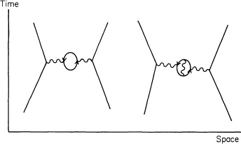
FIGURE 78. The experimentally measured amplitude for an electron to couple with a photon, a mysterious number, e, is a number determined by experiment that includes all the “corrections” for a photon going from point to point in space-time, of which two are shown here. When calculating, we need a number, j, that does not include these corrections, but includes only the photon going directly from point to point. A difficulty exists with computing this j that is similar to the difficulty in computing the value of n.
If there were a definite mathematical connection between n and j on the one hand, and m and e on the other, there would still be no problem: we would simply calculate what values of n and j we need to start with in order to end up with the observed values, m and e. (If our calculations didn’t agree with m and e, we would jiggle the original n and j around until they did.)
Let’s see how we actually calculate m. We write a series of terms that is something like the series we saw for the magnetic moment of the electron: the first term has no couplings—just E (A to B)—and represents an ideal electron going directly from point to point in space-time. The second term has two couplings and represents a photon being emitted and absorbed. Then come terms with four, six, and eight couplings, and so on (some of these “corrections” are shown in Fig. 77).
When calculating terms with couplings, we must consider (as always) all the possible points where couplings can occur, right down to cases where the two coupling points are on top of each other—with zero distance between them. The problem is, when we try to calculate all the way down to zero distance, the equation blows up in our face and gives meaningless answers—things like infinity. This caused a lot of trouble when the theory of quantum electrodynamics first came out. People were getting infinity for every problem they tried to calculate! (One should be able to go down to zero distance in order to be mathematically consistent, but that’s where there is no n or j that makes any sense; that’s where the trouble is.)
Well, instead of including all possible coupling points down to a distance of zero, if one stops the calculation when the distance between coupling points is very small—say, 10-30 centimeters, billions and billions of times smaller than anything observable in experiment (presently 10-16 centimeters)—then there are definite values for n and j that we can use so that the calculated mass comes out to match the m observed in experiments, and the calculated charge matches the observed charge, e. Now, here’s the catch: if somebody else comes along and stops their calculation at a different distance—say, 10-40 centimeters—their values for n and j needed to get the same m and e come out different!
Twenty years later, in 1949, Hans Bethe and Victor Weisskopf noticed something: if two people who stopped at different distances to determine n and j from the same m and e then calculated the answer to some other problem—each using the appropriate but different values for n and j—when all the arrows from all the terms were included, their answers to this other problem came out nearly the same! In fact, the closer to zero distance that the calculations for n and j were stopped, the better the final answers for the other problem would agree! Schwinger, Tomonaga, and I independently invented ways to make definite calculations to confirm that it is true (we got prizes for that). People could finally calculate with the theory of quantum electrodynamics!
So it appears that the only things that depend on the small distances between coupling points are the values for n and j—theoretical numbers that are not directly observable anyway; everything else, which can be observed, seems not to be affected.
The shell game that we play to find n and j is technically called “renormalization.” But no matter how clever the word, it is what I would call a dippy process! Having to resort to such hocus-pocus has prevented us from proving that the theory of quantum electrodynamics is mathematically self-consistent. It’s surprising that the theory still hasn’t been proved self-consistent one way or the other by now; I suspect that renormalization is not mathematically legitimate. What is certain is that we do not have a good mathematical way to describe the theory of quantum electrodynamics: such a bunch of words to describe the connection between n and j and m and e is not good mathematics.1
There is a most profound and beautiful question associated with the observed coupling constant, e—the amplitude for a real electron to emit or absorb a real photon. It is a simple number that has been experimentally determined to be close to –0.08542455. (My physicist friends won’t recognize this number, because they like to remember it as the inverse of its square: about 137.03597 with an uncertainty of about 2 in the last decimal place. It has been a mystery ever since it was discovered more than fifty years ago, and all good theoretical physicists put this number up on their wall and worry about it.)
Immediately you would like to know where this number for a coupling comes from: is it related to pi, or perhaps to the base of natural logarithms? Nobody knows. It’s one of the greatest damn mysteries of physics: a magic number that comes to us with no understanding by man. You might say the “hand of God” wrote that number, and “we don’t know how He pushed His pencil.” We know what kind of a dance to do experimentally to measure this number very accurately, but we don’t know what kind of a dance to do on a computer to make this number come out—without putting it in secretly!
A good theory would say that e is the square root of 3 over 2 pi squared, or something. There have been, from time to time, suggestions as to what e is, but none of them has been useful. First, Arthur Eddington proved by pure logic that the number the physicists like had to be exactly 136, the experimental number at that time. Then, as more accurate experiments showed the number to be closer to 137, Eddington discovered a slight error in his earlier argument, and showed by pure logic again that the number had to be the integer 137! Every once in a while, someone notices that a certain combination of pi’s and e’s (the base of the natural logarithms), and 2’s and 5’s produces the mysterious coupling constant, but it is a fact not fully appreciated by people who play with arithmetic that you would be surprised how many numbers you can make out of pi’s and e’s and so on. Therefore, throughout the history of modern physics, there has been paper after paper by people who have produced an e to several decimal places, only to have the next round of improved experiments disagree with it.
Even though we have to resort to a dippy process to calculate j today, it’s possible that someday a legitimate mathematical connection between j and e will be found. That would mean that; is the mysterious number, and from it comes e. In such a case there would doubtless be another batch of papers that tell us how to calculate j “with our bare hands,” so to speak, proposing that j is 1 divided by 4 * pi, or something.
That exposes all the problems associated with quantum electrodynamics.
When I planned these lectures, I intended to concentrate only on the part of physics that we know very well—to describe it fully and to say no more. But now that we’ve come this far, being a professor (which means having the habit of not being able to stop talking at the right time), I cannot resist telling you something about the rest of physics.
First, I must immediately say that the rest of physics has not been checked anywhere nearly as well as electrodynamics: some of the things I’m going to tell you are good guesses, some are partly worked-out theories, and others are pure speculation. Therefore this presentation is going to look like a relative mess, compared to the other lectures; it will be incomplete and lacking in many details. Nevertheless, it turns out that the structure of the theory of QED serves as an excellent basis for describing other phenomena in the rest of physics.
I’ll begin by talking about protons and neutrons, which make up the nuclei of atoms. When protons and neutrons were first discovered it was thought that they were simple particles, but very soon it became clear that they were not simple—simple in the sense that their amplitude to go from one point to another could be explained by the formula E (A to B), but with a different number for n stuck in. For example, the proton has a magnetic moment that, if calculated in the same way as for the electron, should be close to 1. But in fact, experimentally it comes out completely crazy—2.79! Therefore it was soon realized that something’s going on inside the proton that is not accounted for in the equations of quantum electrodynamics. And the neutron, which should have no magnetic interaction at all if it is really neutral, has a magnetic moment of about –1.93! So it was known for a long time that something fishy is going on inside the neutron as well.
There was also the problem of what holds the neutrons and protons together inside the nucleus. It was realized right away that it could not be the exchange of photons, because the forces holding the nucleus together were much stronger—the energy required to break up a nucleus is much greater than that required to knock an electron away from an atom in the same proportion that an atomic bomb is more destructive than dynamite: exploding dynamite is a rearrangement of the electron patterns, while an exploding atomic bomb is a rearrangement of the proton-neutron patterns.
To find out more about what holds the nuclei together, many experiments were made in which protons with higher and higher energies were smashed into nuclei. It was expected that only protons and neutrons would come out. But when the energies became sufficiently large, new particles came out. First there were pions, then lambdas, and sigmas, and rhos, and they ran out of the alphabet. Then came particles with numbers (their masses), such as sigma 1190 and sigma 1386. It soon became clear that the number of particles in the world was open-ended, and depended on the amount of energy used to break apart the nucleus. There are over four hundred such particles at present. We can’t accept four hundred particles; that’s too complicated!2
Great inventors like Murray Gell-Mann nearly went crazy trying to figure out the rules by which all these particles behave, and in the early 1970s they came up with the quantum theory of strong interactions (or “quantum chromo-dynamics”), whose main actors are particles called “quarks.” All of the particles made of quarks come in two classes: some, like the proton and neutron, are made out of three quarks (and go by the horrible name of “baryons”); others, such as the pions, are made of a quark and an anti-quark (and are called “mesons”).
Let me make a table of the fundamental particles as they appear today (see Fig. 79). I’ll begin with the particles that go from point to point according to the formula E(A to B)—modified by the same kind of polarization rules as an electron—called “spin 1/2” particles. The first of these particles is the electron, and its mass number is 0.511 in units that we use all the time, called MeV.3
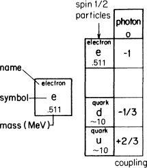
FIGURE 79. Our list of all the particles in the world begins with “spin 1/2” particles: the electron (with a mass of 0.511 MeV), and two “flavors” of quarks, d and u (both with a mass of about 10 MeV). Electrons and quarks have a “charge”—that is, they couple with photons in the following amounts (in terms of the coupling constant, –j): –1, –1/3, and +2/3.
Under the electron I will leave a space (to be occupied later), and under that I will list two types of quarks—the d and the u. The mass of these quarks is not exactly known; a good guess is around 10 MeV for each one. (The neutron is slightly heavier than the proton, which seems to imply—as you will see in a moment—that the d quark is somewhat heavier than the u quark.)
Next to each particle I will list its charge, or coupling constant, in terms of –j, the number for couplings with photons with its sign reversed. This makes the charge for the electron –1, consistent with a convention started by Benjamin Franklin that we’ve been stuck with ever since. For the d quark the amplitude to couple with a photon is –1/3, and for the u quark it is +2/3. (Had Benjamin Franklin known about quarks, he might have at least made the charge of an electron -3!)
Now, the charge of a proton is +1, and a neutron’s charge is zero. With some fiddling about with the numbers, you can see that a proton—made of three quarks—must be two u’s and a d, while a neutron—also made of three quarks—must be two d’s and a u (see Fig. 80).
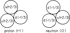
FIGURE 80. All particles made of quarks come in one of only two possible classes: those made of a quark and an anti-quark, and those made of three quarks, of which the proton and the neutron are the most common examples. The charge of the d and u quarks combine to make +1 for the proton and zero for the neutron. The fact that the proton and neutron are made of charged particles going around inside them gives a clue as to why the proton has a magnetic moment higher than 1, and why the supposedly neutral neutron has a magnetic moment at all.
What holds the quarks together? Is it the photons going back and forth? (Because a d quark has a charge of –1/3 and a u quark has a charge of +2/3, quarks, as well as electrons, emit and absorb photons.) No, these electrical forces are far too weak to do that. Something else has been invented to go back and forth and hold quarks together; something called “gluons.”4 Gluons are an example of another type of particle called “spin 1” (as are photons); they go from point to point with an amplitude determined by exactly the same formula as for photons, P(A to B). The amplitude for gluons to be emitted or absorbed by quarks is a mysterious number, g, that is much larger than j (see Fig. 81).
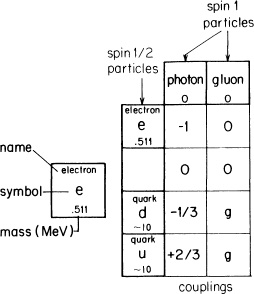
FIGURE 81. “Gluons” hold quarks together to make protons and neutrons, and indirectly account for the fact that protons and neutrons hold themselves together in the nucleus of an atom. Gluons hold quarks together with forces much stronger than electrical forces. The coupling constant of gluons, g, is much larger than j, which makes the calculation of terms with couplings in them much more difficult: the best accuracy that can be hoped for so far is only 10%.
The diagrams we make of quarks exchanging gluons are very similar to the pictures we draw for electrons exchanging photons (see Fig. 82). So similar, in fact, that you might say that the physicists have no imagination—that they just copied the theory of quantum electrodynamics for the strong interactions! And you’re right: that’s what we did, but with a little twist.
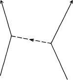
FIGURE 82. The diagram of one way that two quarks can exchange a gluon is so similar to a diagram of two electrons exchanging a photon that you might think the physicists just copied the theory of quantum electrodynamics for the “strong interactions” holding the quarks inside protons and neutrons. Well, they did—almost.
The quarks have an additional type of polarization that is not related to geometry. The idiot physicists, unable to come up with any wonderful Greek words anymore, call this type of polarization by the unfortunate name of “color,” which has nothing to do with color in the normal sense. At a particular time, a quark can be in one of three conditions, or “colors”—R, G, or B (can you guess what they stand for?). A quark’s “color” can be changed when the quark emits or absorbs a gluon. The gluons come in eight different types, according to the “colors” they can couple with. For example, if a red quark changes to green, it emits a red-antigreen gluon—a gluon that takes the red from the quark and gives it green (“antigreen” means the gluon is carrying green in the opposite direction). This gluon could be absorbed by a green quark, which changes to red (see Fig. 83). There are eight different possible gluons, such as red-antired, red-antiblue, red-antigreen, and so on (you’d think there’d be nine, but for technical reasons, one is missing). The theory is not very complicated. The complete rule of gluons is: gluons couple with things having “color”—it just requires a little bookkeeping to keep track of where the “colors” go.
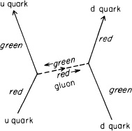
FIGURE 83. Gluon theory differs from electrodynamics in that gluons couple with things that are “colored” (in one of three possible conditions—“red,” “green,” and “blue”). Here, a red u quark changes to green by emitting a red-antigreen gluon that is absorbed by a green d quark changing to red. (If the “color” is being carried backwards in time, it takes the prefix “anti.”)
There is, however, an interesting possibility created by this rule: gluons can couple with other gluons (see Fig. 84). For instance, a green-antiblue gluon meeting a red-antigreen gluon results in a red-antiblue gluon. Gluon theory is very simple—you just make the diagram and follow the “colors.” The strengths of the couplings in all the diagrams is determined from the coupling constant for gluons, g.
Gluon theory is really not a great deal different in form from quantum electrodynamics. How, then, does it compare with experiment? For example, how does the observed magnetic moment of the proton compare with the value calculated from the theory?
The experiments are very accurate—they show the magnetic moment to be 2.79275. At the very best, the theory can only come up with 2.7 plus or minus 0.3—if you’re sufficiently optimistic about the accuracy of your analysis—an error of 10% which is 10,000 times less accurate than experiment! We have a simple, definite theory that is supposed to explain all the properties of protons and neutrons, yet we can’t calculate anything with it, because the mathematics is too hard for us. (You can guess what I’m working on, and I’m not getting anywhere.) The reason we can’t calculate to any great accuracy is because the coupling constant for gluons, g, is so much larger than for electrons. Terms with two, four, and even six couplings are not just minor corrections to the main amplitude; they represent considerable contributions that can’t be ignored. Thus there are arrows from so many different possibilities that we haven’t been able to organize them in a reasonable way to find out what the final arrow is.
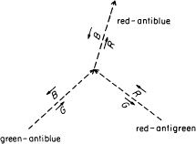
FIGURE 84. Since gluons are themselves “colored,” they can couple to each other. Here a green-antiblue gluon couples with a red-antigreen gluon to form a red-antiblue gluon. Gluon theory is easy to understand—you just follow the “colors.”
In books it says that science is simple: you make up a theory and compare it to experiment; if the theory doesn’t work, you throw it away and make a new theory. Here we have a definite theory and hundreds of experiments, but we can’t compare them! It’s a situation that has never before existed in the history of physics. We’re boxed in, temporarily, unable to come up with a method of calculation. We’re snowed under by all the little arrows.
Despite our difficulties in calculating with the theory, we do understand some things qualitatively about quantum chromodynamics (strong interactions of quarks and gluons). The objects made of quarks that we see are “colored” neutral: groups of three quarks contain one quark of each “color,” and quark-antiquark pairs have an equal amplitude to be red-antired, green-antigreen, or blue-antiblue. We also understand why quarks can never be produced as individual particles—why, no matter how much energy is used to hit a nucleus against a proton, instead of seeing individual quarks come out, we see a jet of mesons and baryons (quark-antiquark pairs and groups of three quarks).
Quantum chromodynamics and quantum electrodynamics aren’t all there is to physics. According to them, a quark cannot change its “flavor”: once a u quark, always a u quark; once a d quark, always a d quark. But Nature behaves differently, sometimes. There is a form of radioactivity that happens slowly—the kind that people worry about leaking out of nuclear reactors—called beta decay, which involves a neutron changing into a proton. Since a neutron consists of two d’s and a u-type quark while a proton is made of two u’s and a d, what really happens is that one of the neutron’s d-type quarks changes into a u-type quark (see Fig. 85). Here’s how it happens: the d quark emits a new thing like a photon called a W, which has a coupling with an electron and with another new particle called an anti-neutrino, a neutrino going backwards in time. The neutrino is another spin 1/2 type particle (like the electron and the quarks), but it has no mass and no charge (it does not interact with photons). It also does not interact with gluons; it only couples with the W (see Fig. 86).
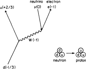
FIGURE 85. When a neutron disintegrates into a proton (a process called “beta decay”), the only thing that changes is the “flavor” of one quark—from d to u—with an electron and an anti-neutrino coming out. This process happens relatively slowly, so an intermediate particle (called a “W-intermediate-boson”) with a very high mass (about 80,000 MeV) and a charge of –1 was proposed.
The W is a spin 1 type particle (like the photon and the gluon), that changes the “flavor” of a quark and takes away its charge—the d, charged –1/3, changes into a u, charged +2/3, a difference of –1. (It doesn’t change the quark’s “color.”) Because the W- takes away a charge of –1 (and its anti-particle, the W+, takes away a charge of +1), it can also couple with a photon. Beta decay takes much longer than the interactions of photons and electrons, so it is thought that the W must have a very high mass (about 80,000 MeV), unlike the photon and gluon. We have not been able to see the W by itself because of the very high energy required to knock loose a particle with such a very high mass.5
There is another particle, which we could think of as a neutral W, called Z0. The Z0 does not change the charge of a quark, but does couple with a d quark, a u quark, an electron, or a neutrino (see Fig. 87). This interaction has the misleading name of “neutral currents,” and caused a lot of excitement when it was discovered a few years ago.
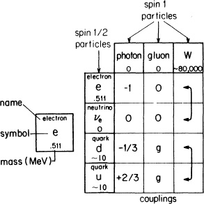
FIGURE 86. The W couples with the electron and neutrino on the one hand, and the d and u quark on the other.
The theory of W’s is nice and neat if you allow for a three-way coupling between the three types of W’s (see Fig. 88). The observed coupling constant for W’s is much the same as that for the photon—in the neighborhood of j. Therefore the possibility exists that the three W’s and the photon are all different aspects of the same thing. Stephen Weinberg and Abdus Salam tried to combine quantum electrodynamics with what’s called the “weak interactions” (interactions with W’s) into one quantum theory, and they did it. But if you just look at the results they get you can see the glue, so to speak. It’s very clear that the photon and the three W’s are interconnected somehow, but at the present level of understanding, the connection is difficult to see clearly—you can still see the “seams” in the theories; they have not yet been smoothed out so that the connection becomes more beautiful and, therefore, probably more correct.
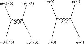
FIGURE 87. When there is no change in the charge of any of the particles, the W also has no charge (it is called Z0 in this case). Such interactions are called “neutral currents.” Two possibilities are shown here.
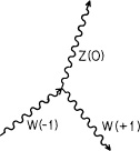
FIGURE 88. A coupling between a W-1, its anti-particle (a W+1, and a neutral W (Z0) is possible. The coupling constant for W’s is in the neighborhood of j, suggesting that W’s and photons may be different aspects of the same thing.
So there you are: quantum theory has three main types of interaction—the “strong interactions” of quarks and gluons, the “weak interactions” of the W’s, and the “electrical interactions” of photons. The only particles in the world (according to this picture) are quarks (in “flavors” u and d with three “colors” each), gluons (eight combinations of R, G, and B), W’s (charged ± 1 and 0), neutrinos, electrons, and photons—about twenty different particles of six different types (plus their anti-particles). That’s not so bad—about twenty different particles—except that’s not all.
As nuclei were hit with protons of higher and higher energies, new particles kept coming out. One such particle was the muon, which is in every way exactly the same as the electron, except that its mass is much higher—105.8 MeV, compared to 0.511 for the electron, or about 206 times heavier. It’s just as if God wanted to try out a different number for the mass! All of the properties of the muon are completely describable by the theory of electrodynamics—the coupling constant j is the same and E(A to B) is the same; you just put in a different value for n.6
Because the muon has a mass about 200 times higher than the electron, the “stopwatch hand” for a muon turns 200 times more rapidly than that of an electron. This has enabled us to test whether electrodynamics still behaves according to the theory at distances 200 times smaller than we’ve been able to test before—although these distances are still more than eighty decimal places larger than the distances at which the theory alone might run into trouble with infinities (see footnote on p. 129).
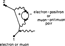
FIGURE 89. In the process of bombarding nuclei with protons of higher and higher energy, new particles appear. One of these particles is the muon, or heavy electron. The theory describing the muon’s interactions is exactly the same as for the electron, except that you just put in a higher number for n into E(A to B). The magnetic moment of a muon should be slightly different than that of an electron because of two particular alternatives: when the electron emits a photon that disintegrates into an electron-positron or muon-antimuon pair, the disintegration creates a pair that is close to or much heavier in mass than the electron. On the other hand, when the muon emits a photon that disintegrates into a muon-antimuon or positron-electron pair, this pair is close to or much lighter in mass than the muon. Experiments confirm this slight difference.
We have learned that an electron can couple with a W (see Fig. 85). When a d-quark changes into a u-quark, emitting a W, can the W then couple with a muon instead of an electron? Yes (see Fig. 90). And what about the anti-neutrino? In the case of the W coupling with a muon, a particle called a mu-neutrino takes the place of the ordinary neutrino (which we will now call an electron neutrino). So now our table of particles has two additional particles next to the electron and the neutrino—the muon and the mu-neutrino.
What about the quarks? Very early on, particles were known that had to be made of heavier quarks than u or d. Thus a third quark, called s (for “strange”) was included in the list of fundamental particles. The s quark has a mass of about 200 MeV, compared to about 10 MeV for the u and d quarks.
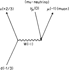
FIGURE 90. The W has an amplitude to emit a muon instead of an electron. In this case a mu-neutrino takes the place of an electron-neutrino.
For many years we thought that there were just three “flavors” of quarks—u, d, and s—but in 1974 a new particle called a psi-meson was discovered that could not be made out of the three quarks. There was also a very good theoretical argument that there had to be a fourth quark, coupled to the s quark by a W in the same way that the u and d quark are coupled (see Fig. 91). The “flavor” of this quark is called c, and I haven’t got the guts to tell you what c stands for, but you may have read it in the newspaper. The names are getting worse and worse!
This repetition of particles with the same properties but heavier masses is a complete mystery. What is this strange duplication of the pattern? As Professor I. I. Rabi said of the muon when it was discovered, “Who ordered that?”
Recently another repetition of the list has begun. As we go to higher and higher energies, Nature seems to keep piling on these particles as if to drug us. I have to tell you about them because I want you to see how apparently complicated the world really looks. It would be very misleading if I were to give you the impression that since we’ve solved 99% of the phenomena in the world with electrons and photons, that the other 1% of the phenomena will take only 1% as many additional particles! It turns out that to explain that last 1%, we need ten or twenty times as many additional particles.
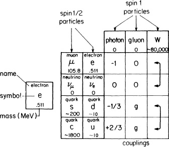
FIGURE 91. Nature seems to be repeating the spin 1/2 particles. In addition to the muon and mu-neutrino, there are two new quarks—s and c—that have the same charge but higher masses than their counterparts in the next column.
So here we go again: with even higher energies used in the experiments, an even heavier electron, called the “tau,” has been found; it has a mass of about 1,800 MeV, heavy as two protons! A tau-neutrino has also been inferred. And now a funny particle has been found implying a new “flavor” of quark—this time it’s “b,” for “beauty,” and it has a charge of –1/3 (see Fig. 92). Now, I want you to become high-class, fundamental theoretical physicists for a moment, and predict something: a new flavor of quark will be found, called__ (for “____”), with a charge of__, a mass of__ MeV—and we certainly hope it’s true that it’s there!7
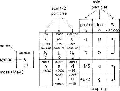
FIGURE 92. Here we go again! Another repetition of the spin 1/2 particles has begun at even higher energies. This repetition will be complete if a particle with the right properties to imply the existence of a new flavor of quark is found. Meanwhile, preparations are underway to look for the beginning of yet another repetition at even higher energies. What causes these repetitions is a complete mystery.
Meanwhile, experiments are being done to see if the cycle repeats yet again. At the present time machines are being built to look for an even heavier electron than the tau. If the mass of this supposed particle is 100,000 MeV, they won’t be able to produce it. If it is around 40,000 MeV, they might make it.
Mysteries like these repeating cycles make it very interesting to be a theoretical physicist: Nature gives us such wonderful puzzles! Why does She repeat the electron at 206 times and 3,640 times its mass?
I’d like to make one last remark to make things absolutely complete about the particles. When a d quark coupling to a W changes into a u quark, it also has a small amplitude to change into a c quark instead. When a u quark goes to a d quark, it also has a small amplitude to change into an s quark, and an even smaller amplitude to change into a b quark (see Fig. 93). Thus the W “screws things up” a little bit and allows quarks to change from one column of the table to another. Why the quarks have these relative proportions for their amplitude to change to another type of quark is utterly unknown.
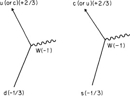
FIGURE 93. A d quark has a small amplitude to change into a c quark instead of a u quark, and an s quark has a small amplitude to change into a u quark instead of a c quark, with the emission of a W in both cases. Thus the W seems to be able to change a quark’s flavor from one column of the table to another (see Fig. 92).
So that’s everything about the rest of quantum physics. It’s a terrible mix-up, and you might say it’s a hopeless mess physics has got itself worked into. But it has always looked like this. Nature has always looked like a horrible mess, but as we go along we see patterns and put theories together; a certain clarity comes and things get simpler. The mess I just showed you is much smaller than the mess I would have had to make ten years ago, telling you about the more than four hundred particles. And think about the mess at the beginning of this century, when there was heat, magnetism, electricity, light, X-rays, ultraviolet rays, indices of refraction, coefficients of reflection and other properties of various substances, all of which we have since put together into one theory, quantum electrodynamics.
I would like to emphasize something. The theories about the rest of physics are very similar to the theory of quantum electrodynamics: they all involve the interaction of spin 1/2 objects (like electrons and quarks) with spin 1 objects (like photons, gluons, or W’s) within a framework of amplitudes by which the probability of an event is the square of the length of an arrow. Why are all the theories of physics so similar in their structure?
There are a number of possibilities. The first is the limited imagination of physicists: when we see a new phenomenon we try to fit it into the framework we already have—until we have made enough experiments, we don’t know that it doesn’t work. So when some fool physicist gives a lecture at UCLA in 1983 and says, “This is the way it works, and look how wonderfully similar the theories are,” it’s not because Nature is really similar; it’s because the physicists have only been able to think of the same damn thing, over and over again.
Another possibility is that it is the same damn thing over and over again—that Nature has only one way of doing things, and She repeats her story from time to time.
A third possibility is that things look similar because they are aspects of the same thing—some larger picture underneath, from which things can be broken into parts that look different, like fingers on the same hand. Many physicists are working very hard trying to put together a grand picture that unifies everything into one super-duper model. It’s a delightful game, but at the present time none of the speculators agree with any of the other speculators as to what the grand picture is. I am exaggerating only slightly when I say that most of these speculative theories have no more deep sense to them than your guess about the possibility of a t quark, and I guarantee you that they are no better at guessing the mass of a t quark than you are!
For example, it appears that the electron, the neutrino, the d quark, and the u quark all go together—indeed, the first two couple with the W, as do the last two. At present it is thought that a quark can only change “colors” or “flavors.” But perhaps a quark could disintegrate into a neutrino by coupling with an undiscovered particle. Nice idea. What would happen? That would mean protons are unstable.
Somebody makes up a theory: The proton is unstable. They make a calculation and find that there would be no protons in the universe anymore! So they fiddle around with the numbers, putting a higher mass into the new particle, and after much effort they predict that the proton will decay at a rate slightly less than the last measured rate the proton has been shown not to decay at.
When a new experiment comes along and measures the proton more carefully, the theories adjust themselves to squeeze out from the pressure. The most recent experiment showed that the proton doesn’t decay at a rate that is five times slower than what was predicted in the last stand of the theories. What do you think happened? The phoenix just rose again with a new modification of the theory that requires even more accurate experiments to check it. Whether the proton decays or not is not known. To prove that it does not decay is very difficult.
In all of these lectures I did not discuss gravitation. The reason is, gravitational influence between objects is extremely small: it is a force that is weaker by 1 followed by 40 zeros than the electrical force between two electrons (perhaps it’s 41 zeros). In matter, nearly all of the electrical forces are spent holding the electrons close to the nucleus of their atom, creating a finely balanced mixture of pluses and minuses that cancel out. But with gravitation, the only force is attraction, and it keeps adding and adding as there are more and more atoms until at last, when we get to these ponderously large masses that we are, we can begin to measure the effects of gravity—on planets, on ourselves, and so on.
Because the gravitational force is so much weaker than any of the other interactions, it is impossible at the present time to make any experiment that is sufficiently delicate to measure any effect that requires the precision of a quantum theory of gravitation to explain it.8 Even though there is no way to test them, there are, nevertheless, quantum theories of gravity that involve “gravitons” (which would appear under a new category of polarizations, called “spin 2”), and other fundamental particles (some with spin 3/2). The best of these theories is not able to include the particles that we do find, and invents a lot of particles that we don’t find. The quantum theories of gravity also have infinities in the terms with couplings, but the “dippy process” that is successful in getting rid of the infinities in quantum electrodynamics doesn’t get rid of them in gravitation. So not only have we no experiments with which to check a quantum theory of gravitation, we also have no reasonable theory.
Throughout this entire story there remains one especially unsatisfactory feature: the observed masses of the particles, m. There is no theory that adequately explains these numbers. We use the numbers in all our theories, but we don’t understand them—what they are, or where they come from. I believe that from a fundamental point of view, this is a very interesting and serious problem.
I’m sorry if all this speculation about new particles confused you, but I decided to complete my discussion of the rest of physics to show you how the character of those laws—the framework of amplitudes, the diagrams that represent the interactions to be calculated, and so on—appears to be the same as for the theory of quantum electrodynamics, our best example of a good theory.
Note Added in Proofreading, November 1984:
Since these lectures were given, suspicious events observed in experiments make it appear possible that some other particle or phenomenon, new and unexpected (and therefore not mentioned in these lectures), may soon be discovered.
Note Added in Proofreading, April 1985:
At this moment, the “suspicous events” mentioned above appear to be a false alarm. The situation no doubt will have changed again by the time you read this book. Things change faster in physics than in the book publishing business.
1 Another way of describing this difficulty is to say that perhaps the idea that two points can be infinitely close together is wrong—the assumption that we can use geometry down to the last notch is false. If we make the minimum possible distance between two points as small as 10-100 centimeters (the smallest distance involved in any experiment today is around 10-16 centimeters), the infinities disappear, all right—but other inconsistencies arise, such as the total probability of an event adds up to slightly more or less than 100%, or we get negative energies in infinitesimal amounts. It has been suggested that these inconsistencies arise because we haven’t taken into account the effects of gravity—which are normally very, very weak, but become important at distances of 10-33 cm.
2 Although many particles come out of the nucleus in high-energy experiments, in low-energy experiments—in more normal conditions—the nuclei are found to contain only protons and neutrons.
3 An MeV is very small—appropriate to such particles—about 1.78 * 10-27 grams.
4 Notice the names: “photon” comes from the Greek word for light; “electron” comes from the Greek word for amber, the beginning of electricity. But as modern physics has progressed, the names of the particles have shown a deteriorating interest in classical Greek until we make up such words as “gluons.” Can you guess why they’re called “gluons?” in fact, d and u stand for words, but I don’t want to confuse you—a d quark is no more “down” than a u quark is “up.” Incidentally, the d-ness or u-ness of a quark is called its “flavor.”
5 After these lectures were given, high enough energies were achieved to produce a W by itself, and its mass was measured to be very close to the value predicted by the theory.
6 The magnetic moment of a muon has been measured very accurately—it has been found to be 1.001165924 (with an uncertainty of 9 in the last digit), while the value for the electron is 1.00115965221 (with an uncertainty of 3 in the last digit). You might be curious as to why the magnetic moment of the muon is slightly higher than that of the electron. One of the diagrams we drew had the electron emitting a photon that disintegrates into a positron-electron pair (see Fig. 89). There is also a small amplitude that the emitted photon could make a muon-antimuon pair, which is heavier than the original electron. This is unsymmetrical, because when the muon emits a photon, if that photon makes a positron-electron pair, that pair is lighter than the original muon. The theory of quantum electrodynamics accurately describes every electrical property of the muon as well as the electron.
7 Since these lectures were given, some evidence has been found for the existence of a t quark with a very high mass—around 40,000 MeV.
8 When Einstein and others tried to unify gravitation with electrodynamics, both theories were classical approximations. In other words, they were wrong. Neither of these theories had the framework of amplitudes that we have found to be so necessary today.