Let's go into the details of what is happening to configure a reinforcement agent using Q-learning. The goal of Q-learning is to create a state–action matrix where a value is assigned for all state–action combinations—that is, if our agent is at any given state, then the values provided determine the action the agent will take to obtain maximum value. We are going to enable the computation of the best policy for our agent by creating a value matrix that provides a calculated value for every possible move:
- To start, we need a set of state and action pairs that all have a value of 0. As a best practice, we will use hashing here, which is a more efficient alternative to large lists for scaling up to more complex environments. To begin, we will load the hash library and then we will use a for loop to populate the hash environment. The for loop starts by getting every unique state from the data, and for every unique state, it then appends every unique action to create all possible state–action pairs and assigns all pairs a value of 0. We generate this hash environment that will hold the values calculated during the Q-learning phase by running the following code:
library(hash)

Q <- hash()

for (i in unique(tictactoe$State)[!unique(tictactoe$State) %in% names(Q)]) {
 Q[[i]] <- hash(unique(tictactoe$Action), rep(0, length(unique(tictactoe$Action))))
}
After running the code, we will see that our Environment pane now looks like the following screenshot:
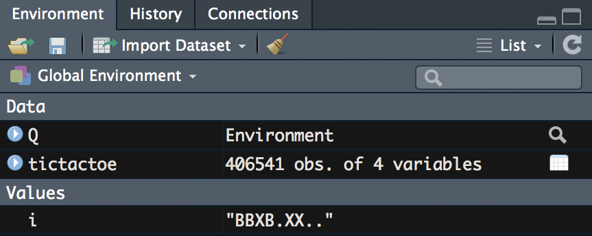
We have a hash environment, Q, that contains every state-action pair.
- The next step is to define the hyperparameters. For now, we will use the default values; however, we will soon tune these to see the impact. We set the hyperparameters to their default values by running the following code:
control = list(
 alpha = 0.1,
 gamma = 0.1,
 epsilon = 0.1
 )
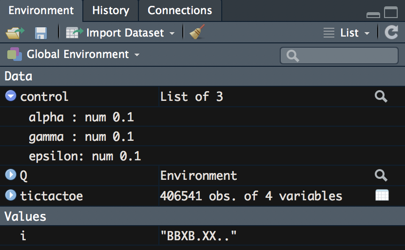
After running the code, we can now see that we have a list with our hyperparameter values in our Environment pane, which now looks like the following:
- Next, we begin to populate our Q matrix. This again takes place within a for loop; however, we will look at one isolated iteration. We start by taking a row and moving the elements from this row to discrete data objects using the following code:
  d <- tictactoe[1, ]
  state <- d$State
  action <- d$Action
  reward <- d$Reward
  nextState <- d$NextState
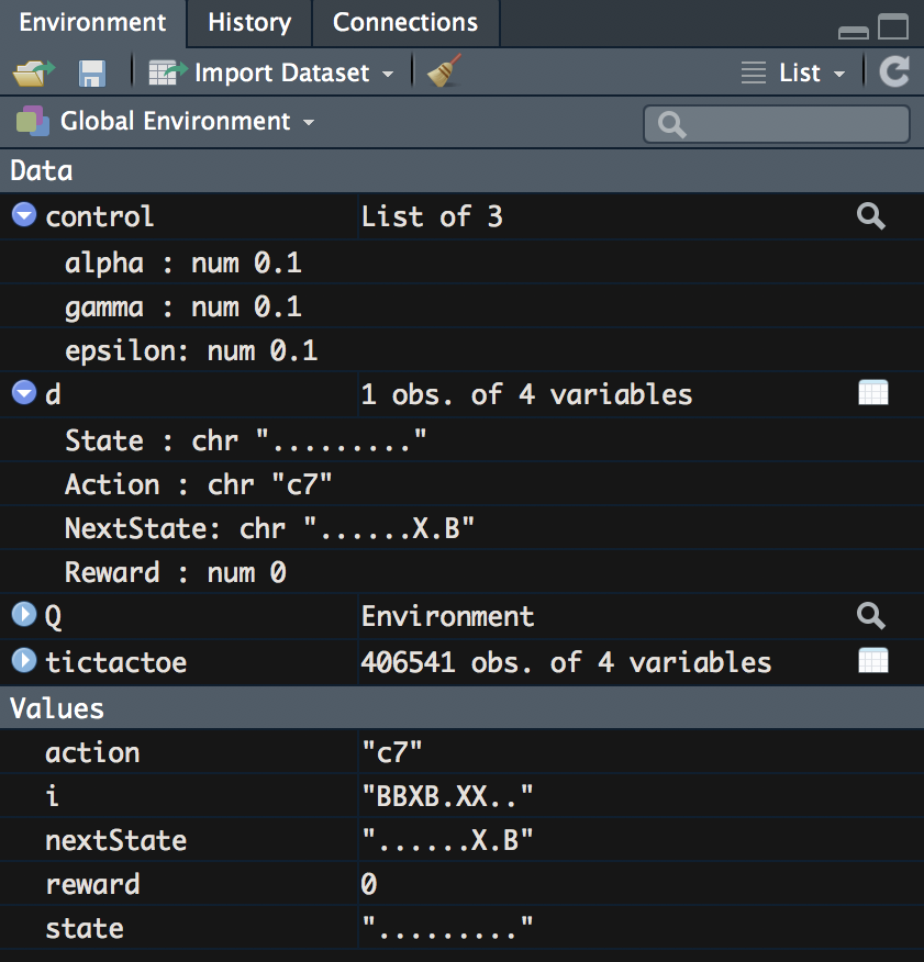
After running the code, we can see the changes to our Environment pane, which now contains the discrete elements from the first row. The Environment pane will look like the following:
- Next, we get a value for the current Q-learning score if there is one. If there isn't a value, then 0 is stored as the current value. We set this initial quality value score by running the following code:
  currentQ <- Q[[state]][[action]]
  if (has.key(nextState,Q)) {
    maxNextQ <- max(values(Q[[nextState]]))
  } else {
    maxNextQ <- 0
  }
After running this code, we now have a value for currentQ, which is 0 in this case because all values in Q for the state '......X.B' are 0, as we have set all values to 0; however, in the next step, we will begin to update the Q values.
- Lastly, we update the Q value by using the Bellman equation. This is also called temporal difference learning. We write out this step for computing values with this equation for R using the following code:
  ## Bellman equation
  Q[[state]][[action]] <- currentQ + control$alpha *
    (reward + control$gamma * maxNextQ - currentQ)

q_value <- Q[[tictactoe$State[1]]][[tictactoe$Action[1]]]
After running the following code, we can pull out the updated value for this state–action pair; we can see it in the field labeled q_value. Your Environment pane will look like the following screenshot:
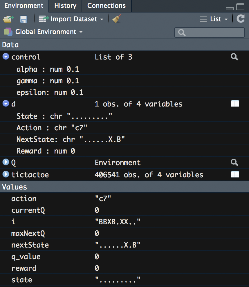
We note here that the q_value is still 0. Why is this the case? If we look at our equation, we will see that the reward is part of the equation and our reward is 0, which makes the entire calculated value 0. As a result, we will not begin to see updated Q values until our code encounters a row with a nonzero reward.
- We can now put all of these steps together and run them over every row to create our Q matrix. We create the matrix of values that we will use to select the policy for optimal strategy by running the following code, which wraps all the previous code together in a for loop:
for (i in 1:nrow(tictactoe) {
d <- tictactoe[i, ]
state <- d$State
action <- d$Action
reward <- d$Reward
nextState <- d$NextState
currentQ <- Q[[state]][[action]]
if (has.key(nextState,Q)) {
maxNextQ <- max(values(Q[[nextState]]))
} else {
maxNextQ <- 0
}
## Bellman equation
Q[[state]][[action]] <- currentQ + control$alpha *
(reward + control$gamma * maxNextQ - currentQ)
}
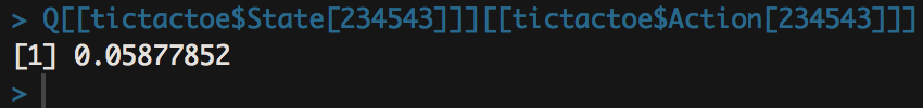
Q[[tictactoe$State[234543]]][[tictactoe$Action[234543]]]
After looping through all the rows, we see that some state–action pairs do now have a value in the Q matrix. Running the following code, we will see the following value printed to our console:
At this point, we have now created our matrix for Q-learning. In this case, we are storing the value in a hash environment with values for every key-value pairing; however, this is equivalent to storing the values in a matrix—it is just more efficient for scaling up later. Now that we have these values, we can compute a policy for our agent that will provide the best path to a reward; however, before we compute this policy, we will make one last set of modifications, and that is to tune the hyperparameters that we set earlier to their default values.