To avoid overfitting, we can use two techniques. The first is adding a dropout layer. The dropout layer will remove a subset of the layer output. This makes the data a little different at every iteration so that the model generalizes better and doesn't fit the solution too specifically to the training data. In the preceding code, we add the dropout layer after the pooling layer:
model <- keras_model_sequential()
model %>%
  layer_conv_2d(filters = 128, kernel_size = c(7,7), input_shape = c(28,28,1), padding = "same") %>%
  layer_activation_leaky_relu() %>%
  layer_max_pooling_2d(pool_size = c(2, 2)) %>%
  layer_dropout(rate = 0.2) %>%
  layer_conv_2d(filters = 64, kernel_size = c(7,7), padding = "same") %>%
  layer_activation_leaky_relu() %>%
  layer_max_pooling_2d(pool_size = c(2, 2)) %>%
  layer_dropout(rate = 0.2) %>%
  layer_conv_2d(filters = 32, kernel_size = c(7,7), padding = "same") %>%
  layer_activation_leaky_relu() %>%
  layer_max_pooling_2d(pool_size = c(2, 2)) %>%
  layer_dropout(rate = 0.2) %>%
  layer_flatten() %>%
  layer_dense(units = 128) %>%
  layer_activation_leaky_relu() %>%
  layer_dropout(rate = 0.2) %>%
  layer_dense(units = 10, activation = 'softmax')

# compile model
model %>% compile(
  loss = 'categorical_crossentropy',
  optimizer = 'adam',
  metrics = 'accuracy'
)
# train and evaluate
model %>% fit(
  train, train_target,
  batch_size = 100,
  epochs = 5,
  verbose = 1,
  validation_data = list(test, test_target)
)
scores <- model %>% evaluate(
  test, test_target, verbose = 1
)
preds <- model %>% predict(test)
predicted_classes <- model %>% predict_classes(test)
caret::confusionMatrix(as.factor(predicted_classes),as.factor(test_target_vector))
The preceding code prints model diagnostic data to our console. Your console will look like the following image:

The preceding code also produces a plot with model performance data. You will see a plot like the following image in your Viewer pane:

The preceding code also produces some performance metrics. The output printed to your console will look like the following image:
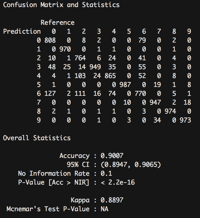
In this case, using this tactic caused our accuracy score to decrease slightly to 90.07%. This could be due to working with a dataset of such small images that the model suffered from the removal of data at every step. With larger datasets, this will likely help make models more efficient and generalize better.
The other tactic for preventing overfitting is using early stopping. Early stopping will monitor progress and stop the model from continuing to train on the data when the model no longer improves. In the following code, we have set the patience argument to 2, which means that the evaluation metric must fail to improve for two epochs in a row.
In the following code, with epochs kept at 5, the model will complete all five rounds; however, if you have time, feel free to run all the preceding code and then, when it is time to fit the model, increase the number of epochs to see when the early stopping function stops the model. We add early stopping functionality to our model using the following code:
model %>% fit(
  train, train_target,
  batch_size = 100,
  epochs = 5,
  verbose = 1,
  validation_data = list(test, test_target),
  callbacks = list(
    callback_early_stopping(patience = 2)
  )
)
From the preceding code, we can deduce the following:
- Using dropout and early stopping, we demonstrated methods for discovering the optimal number of epochs or rounds for our model.
- When thinking of the number of epochs we should use, the goal is twofold.
- We want our model to run efficiently so that we are not waiting for our model to finish running, even though the additional rounds are not improving performance. We also want to avoid overfitting where a model is trained too specifically on the training data and is unable to generalize to new data.
- Dropout helps with the second issue by arbitrarily removing some data on each round. It also introduces randomness that prevents the model from learning too much about the whole dataset.
- Early stopping helps with the first problem by monitoring performance and stopping the model when the model is no longer producing better results for a given length of time.
- Using these two techniques together will allow you to find the epoch number that allows the model to run efficiently and also generalize well.