1 Introduction
Many time series are realizations of nonstationary random processes, hence estimating their time varying spectra may provide insight into the physical processes that give rise to these time series. For example, EEG time series are typically nonstationary, and estimating the time varying spectra based on the EEG of epilepsy patients may lead to methods capable of predicting seizure onset; e.g., see [2]. Similarly, analyzing the time varying spectrum of the Southern Oscillation Index (SOI) may further our knowledge of the frequency of the El Niño Southern Oscillation (ENSO) phenomenon and its impact on global climate; e.g., see [3].
Most established techniques that search for structural breaks in time series, however, may not be able to identify slight frequency changes at the resolution of interest. Of course, the resolution depends on the particular application. The problem is that many of the techniques assume very smooth local spectra and tend to produce overly smooth estimates. The problem of assuming very smooth spectra produces spectral estimates that may miss slight frequency changes because frequencies that are close together will be lumped into one frequency; see Sect. 5 for further details. The goal of this work is to develop techniques that concentrate on detecting slight frequency changes by requiring a high degree of resolution in the frequency domain.
The basic assumptions here are that, conditional on the location and number of segments, the time series is piecewise stationary with each piece having a spectral density. A detailed description of the model is given in Sect. 2. In addition to representing time series that have regime changes, the model can be used to approximate slowly varying processes; e.g., see [1], which uses dyadic segmentation to find the approximate location of breakpoints. The approach taken in [8] was to fit piecewise AR models using minimum description length and a genetic algorithm for solving the difficult optimization problem. [13] proposed nonparametric estimators based on dyadic segmentation and smooth local exponential functions. [15] estimated the log of the local spectrum using a Bayesian mixture of splines. The basic idea of this approach is to first partition the data into small sections. It is then assumed that the log spectral density of the evolutionary process in any given partition is a mixture of individual log spectra. A mixture of smoothing splines model with time varying mixing weights is used to estimate the evolutionary log spectrum. Later, [16] improved on the technique of [15] by adaptively selecting breakpoints.
 , into components of oscillation indexed by frequency
  , and measured in cycles per unit of time, for
  . Given a time series sample,
  , that has been centered by its sample mean, the sample spectral density (or periodogram) is defined in terms of frequency
  :
:
 .
. , of a stationary time series can be defined as the limit (
 ) of
) of ![$$E[I_n(\omega )]$$](../images/461444_1_En_42_Chapter/461444_1_En_42_Chapter_TeX_IEq9.png) , provided that the limit exists; details can be found in
[17, Chap. 4]. It is worthwhile to note that
, provided that the limit exists; details can be found in
[17, Chap. 4]. It is worthwhile to note that  ,
,  , and
, and
 . Thus, the spectral density can be thought of as the variance density of a time series relative to frequency of oscillation. That is, for positive frequencies between 0 and 1/2, the proportion of the variance that can be attributed to oscillations in the data at frequency
  is roughly
  . If the time series
  is white noise, that is,
  is independent of time t, and
  for all
  , then
  . The designation white originates from the analogy with white light and indicates that all possible periodic oscillations are present with equal strength.
2 Model and Existing Methods
 consist of an unknown number of segments, m, and let
  be the unknown location of the end of the jth segment,
  , with
  and
and  . Then conditional on m and
  , we assume that the process
  is piecewise stationary. That is,
 , the processes
  have spectral density
  that may depend on parameters
  , and
, and  if
if ![$$t \in [\xi _{j-1}+1, \xi _{j}]$$](../images/461444_1_En_42_Chapter/461444_1_En_42_Chapter_TeX_IEq32.png) and 0 otherwise.
and 0 otherwise. from process (3), where the number and locations of the stationary segments is unknown. Let
  be the number of observations in the jth segment. We assume that each
  is large enough for the local Whittle likelihood (see
[20]) to provide a good approximation to the likelihood. Given a partition of the time series
  , the jth segment consists of the observations
  ,
,  , with underlying spectral densities
  and periodograms
  , evaluated at frequencies
  ,
,  . For a given partition
  , the approximate likelihood of the time series is given by
![$$\begin{aligned} L(f^\theta _{1},\ldots ,f^\theta _{m} \mid \pmb x, \pmb \xi ) \approx \prod _{j=1}^m (2\pi )^{-n_{j}/2} \prod _{k_j=0}^{n_{j}-1} \exp \Bigl \{-\frac{1}{2}\Bigl [\log f^\theta _{j}(\omega _{k_j})\\ +I_{j}(\omega _{k_j})/f^\theta _{j}(\omega _{k_j})\Bigr ]\Bigr \}. \end{aligned}$$](../images/461444_1_En_42_Chapter/461444_1_En_42_Chapter_TeX_Equ4.png)
2.1 AdaptSpec
The frequency domain approach used in
[16] is a Bayesian method that incorporates (4) with a linear smoothing spline prior on the  for
for  . In addition, a uniform prior is placed on the breakpoints,
  for
for  where
where  is the number of available locations for split point
  , as is the prior on the number of segments,
  for
for  and M is some large but fixed number. The approach uses reversible jump Markov chain Monte Carlo (RJ-MCMC) methods to evaluate the posteriors. The technique is available in an R package called BayesSpec.
2.2 AutoParm
 is piecewise stationary with AR
 behavior in each segment,
  . Then, Minimum Description Length (MDL) as described in
[14] is used to find the best combination of the number of segments, m, the breakpoints
  (or segment sizes
  ), and the orders/estimates of the piecewise AR processes. The idea is to minimize the Code Length (CL) necessary to store the data (i.e., the amount of memory required to encode the data), which leads to a BIC-type criterion to find the model that minimizes
 and
and  maximized value of the usual Gaussian AR(
 ) likelihood for segment
  ,
,
 is the segment’s constant mean value,
  is the corresponding vector of ones, and
  is the usual AR
 variance-covariance matrix corresponding to
  . Because of the Markov structure of AR models, the likelihood has a simple form; see
[6, Prob. 8.7] for details. Fitting the model has to be done via numerical optimization, which is accomplished via a genetic algorithm (a derivative free smart search for minimization based on evolutionary biology concepts). Basic information on genetic algorithms may be obtained from the Mathworks site
[11].
. Because of the Markov structure of AR models, the likelihood has a simple form; see
[6, Prob. 8.7] for details. Fitting the model has to be done via numerical optimization, which is accomplished via a genetic algorithm (a derivative free smart search for minimization based on evolutionary biology concepts). Basic information on genetic algorithms may be obtained from the Mathworks site
[11].2.3 The Problem Is Resolution
The problem with the aforementioned techniques is that they tend to over-smooth the spectral density estimate so that small frequency shifts cannot be detected. Resolution problems were thoroughly discussed in the literature in the latter half of the twentieth century. Some details of the history of the problem as well as a simulation example are given in Sect. 5. For our analysis, we focus on El Niño–Southern Oscillation (ENSO). The Southern Oscillation Index (SOI) measures changes in air pressure related to sea surface temperatures in the central Pacific Ocean. The central Pacific warms every three to seven years due to the El Niño effect, which has been blamed for various global extreme weather events. It has become taken as fact that sometime after 1980, the frequency of the El Niño–La Niña (or ENSO) cycle has increased with the global warming; e.g., see [19].
 . However, assuming that there is one structural break, the posterior distribution of the breakpoints (with a vertical line at the mean) is displayed in the figure.
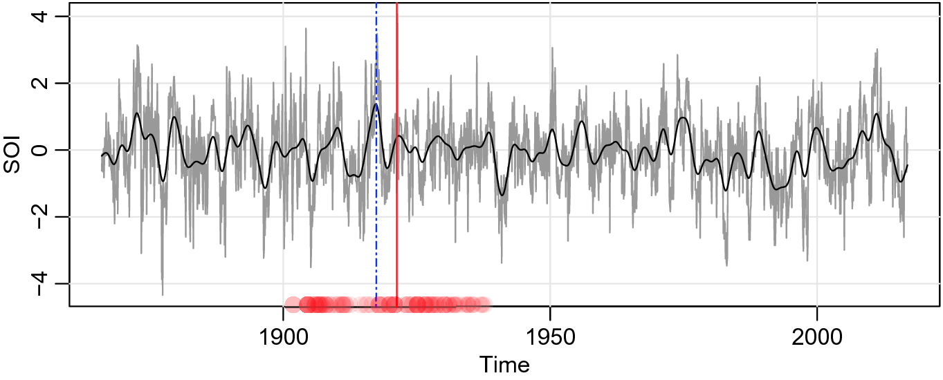
Monthly values of the SOI for years 1866–2017 with breakpoints (vertical lines) determined by AutoParm (- - -) and by AdaptSpec (|). The solid smooth line is the filtered series that exhibits the ENSO cycle. For AdaptSpect,  indicates there is probably not a breakpoint
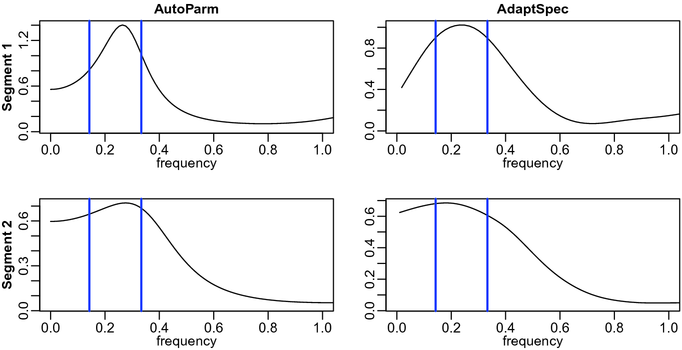
The segmented spectral estimates using AutoParm and AdaptSpec. The vertical lines show the 3–7 7 year cycle known ENSO cycle range. The frequency scale is in years and is truncated at the annual cycle
Figure 2 shows the estimated spectra for each segment for the AutoParm and AdaptSpec techniques. The vertical lines show the 3–7 year cycle known ENSO cycle (see https://www.weather.gov/mhx/ensowhat for more details). Both methods indicate that in the second segment, the ENSO cycle is much more broad, including both slower and faster frequencies than the usual ENSO cycle. One thing that is clear from both methods is that the estimated spectra are too smooth (broad) to reveal if there has been a decisive frequency shift in the ENSO cycle.
3 AutoSpec—Parametric
 with the Whittle likelihood (4) but with
 is the AR polynomial of order
  given by.
 . The basic idea is use peridograms as the data in a move from the time domain to the frequency domain. Another similar method would be to use the Bloomfield EXP model
[5],
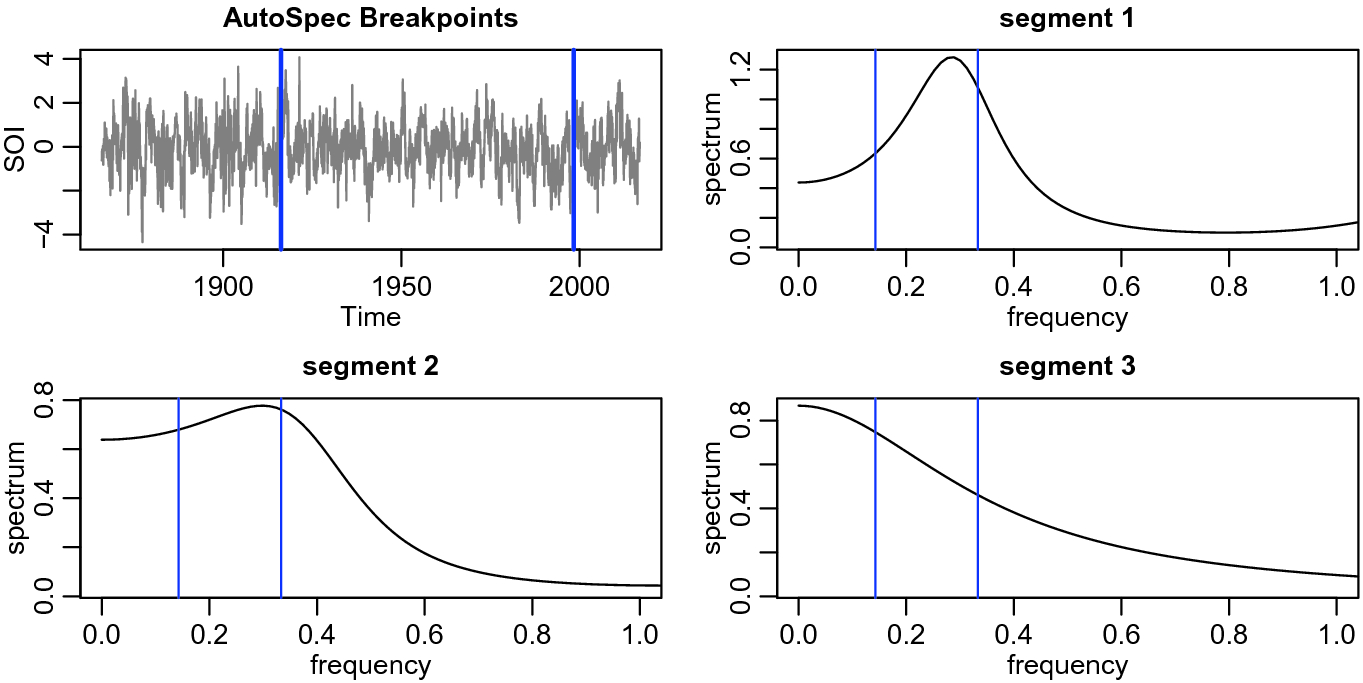
The SOI series with the two breakpoints found using AutoSpec. The individual AR spectral estimates for each of the three segments. The vertical lines show the 3–7 year cycle known ENSO cycle range
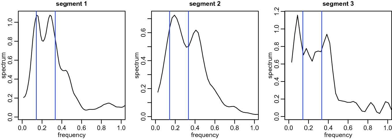
Nonparametric estimates of the spectra in the three segments identified by AutoSpec; compare to Figure 3. The vertical lines show the 3–7 year cycle known ENSO cycle range
4 AutoSpecNP—Nonparametric
 with
with  such that
  , with the bandwidth b chosen by MDL to smooth the periodogram of the fully tapered data and then used the Whittle likelihood for the given spectral estimate. That is, to nonparametrically evaluate the likelihood (4) in each segment
  , use
, use
 are chosen by MDL (similar to AR orders in AutoParm). Here,
  represents the periodogram of the fully cosine tapered data in segment j for
  .
. represents the data in a segment, then they are preprocessed as
  where
where  is the cosine bell taper favored by
[4],
is the cosine bell taper favored by
[4],![$$ h_t=.5\biggl [1+\cos \biggl (\frac{2\pi (t-\overline{t}) }{ n}\biggr )\biggr ]\,, $$](../images/461444_1_En_42_Chapter/461444_1_En_42_Chapter_TeX_Equ12.png)
 and n is the number of observations in that segment. In this case, the periodogram is of the preprocessed data,
  . Figure 5 shows an example of the Bartlett window with
  ; the corresponding spectral window (see
[17, Sect. 4]) of the Bartlett kernel is not very good unless the data are tapered. The spectral window corresponding to the Bartlett kernel with tapering is also displayed in Figure 5.
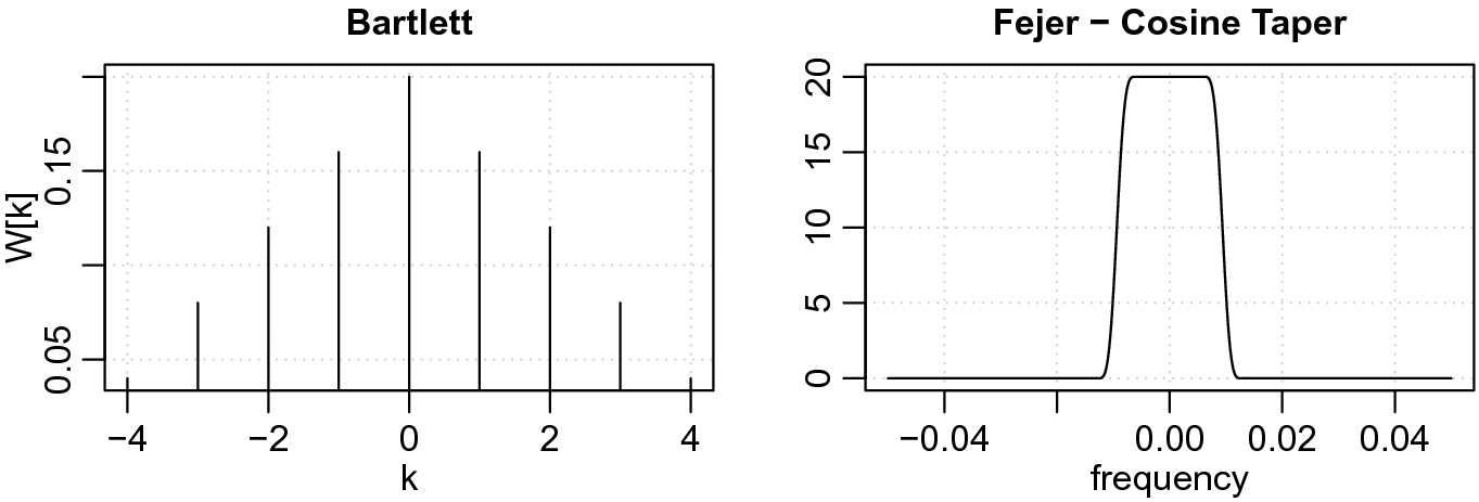
Example of the Bartlett kernel and the corresponding Fejér spectral window when a taper is applied
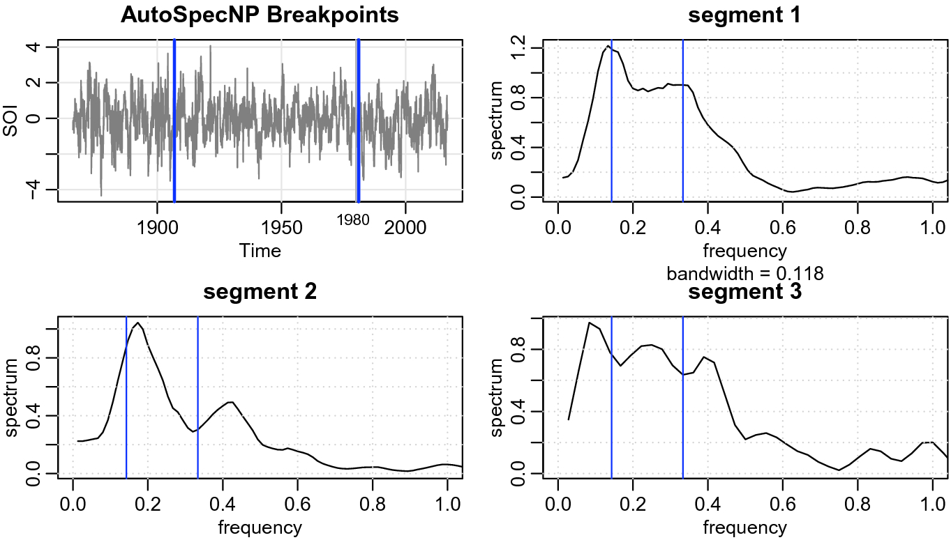
Figure 6 shows the results of the fully nonparametric method. The figure displays the SOI series along with the estimated breakpoints. The fully nonparametric method finds a breakpoint near 1980 as has been suggested by climatologists, initially in [18]. Although the differences in each segment are subtle, this method has enough resolution to distinguish between minor frequency shifts. We may interpret the findings as follows. From 1866 to 1905, the ENSO cycle was a 3–7 year cycle. After that, there appears to be a shift to a higher ENSO cycle of about 2.5 years in addition to the usual 3–7 year cycle. Finally, after 1980, there appears to be a slower cycle introduced into the system. That is, after 1980, the ENSO cycle included a much slower cycle that indicates that El Niño events tend to be longer, but not faster than 2.5 years.
5 Spectral Resolution and a Simulation
As previously stated, the problem of resolution was discussed in the literature in the latter half of the twentieth century; e.g.,
[9, 10]. The basic rule of thumb is that the achievable frequency resolution,  should be approximately the reciprocal of the observational time interval,
  of the data,
  Two signals can be as close as
  apart before there is significant overlap in the transform and the separate peaks are no longer distinguishable.

 ,
,  , and
, and  for
for  are independent i.i.d. standard normals. The difference between the two halves of the data is that
  is a modulated version of
  . Modulation is a common occurrence in many signal processing applications, e.g., EEG (see
[12]). In addition, note that
. Modulation is a common occurrence in many signal processing applications, e.g., EEG (see
[12]). In addition, note that![$$ X_{1t}= \cos (2\pi [\omega +\delta ]\, t) + \cos (2\pi [\omega -\delta ]\, t) + Z_{1t}\,, $$](../images/461444_1_En_42_Chapter/461444_1_En_42_Chapter_TeX_Equ13.png)
 is distinguishable by twin peaks in the frequency domain.
Realization of (9) showing the true breakpoint as a solid vertical line; the dashed vertical line shows the breakpoint identified by AutoSpecNP
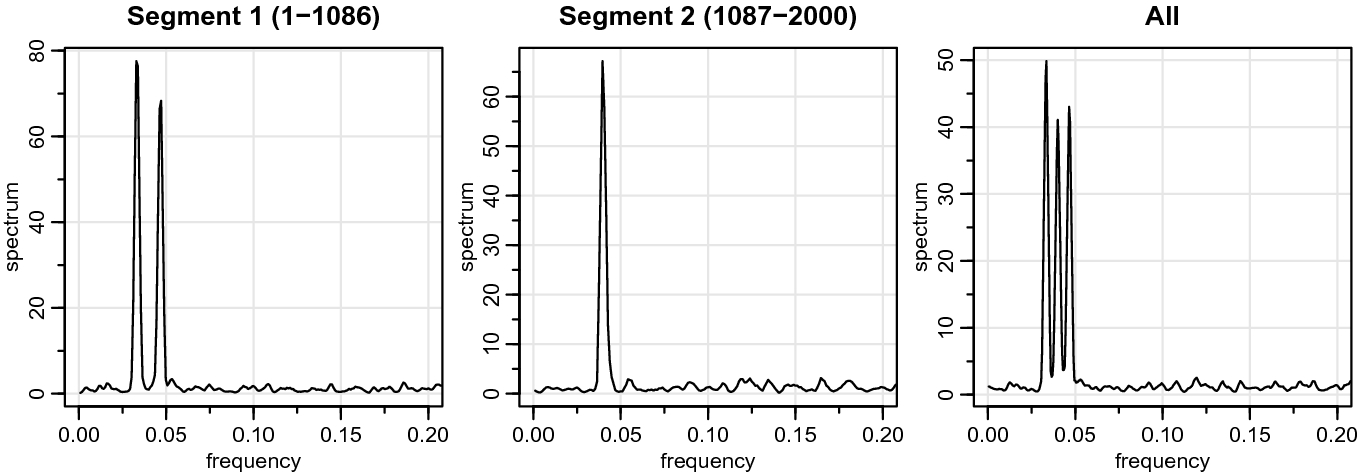
The results of running AutoSpecNP on the data  , which finds one breakpoint at
  . The figures are the estimated AutoSpecNP spectra for each identified segment and the estimate (8) with
  on all the data
Figure 7 shows a realization of  with the changepoint marked. The figure also displays the breakpoint
  identified by AutoSpecNP. We note, however, that AutoSpec and AutoParm do not identify any breakpoints.
Figure 8 shows the results of running AutoSpecNP described in Sect. 4 on the data  . As seen from the figure, the procedure is able to distinguish between the two processes (with a breakpoint at
  ). The method works because the procedure allows very limited to no smoothing of the periodogram. In addition to showing the spectral estimates of each segment, the figure also displays the estimate (8) with
  on the entire realization of
  . This figure helps in realizing why the method works.