1 Introduction
The choice between parametric and nonparametric density estimates is a topic frequently encountered by practitioners. The parametric (maximum likelihood, ML) approach is a natural first choice under strong evidence about the underlying density. However, estimation of normal mixture densities with unknown number of mixture components can become very complicated. Specifically, misidentification of the number of components greatly impairs the performance of the ML estimate and acts incrementally to the usual convergence issues of this technique, e.g., [11]. A robust nonparametric alternative, immune to the above problems is the classical kernel density estimate (kde).
The purpose of this work is to investigate under which circumstances one would prefer to employ the ML or the kde. A goodness-of-fit test is introduced based on the Integrated Squared Error (ISE) which measures the distance between the true curve and the proposed parametric model. Section 2 introduces the necessary notation and formulates the goodness-of-fit test. Its asymptotic distribution is discussed in Sect. 3 together with the associated criteria for acceptance or rejection of the null. An example is provided in Sect. 4. All proofs are deferred to the last Section.
2 Setup and Notation
 denote the standard normal density and
  its scaled version. Let
  where for each
  ,
,  and
and  where each
  . Let also
  be a vector of positive parameters summing to one. The finite positive integer k denotes the number of mixing components. Then,
 , scale parameter
  , and mixing parameter
  . The number of mixing components k is estimated prior and separately to estimation of
  . Thus it is considered as a fixed constant in the process of ML estimation. Popular estimation methods for k include clustering as in
[14] or by multimodality hypothesis testing as in
[6] among many others. Regarding
. Thus it is considered as a fixed constant in the process of ML estimation. Popular estimation methods for k include clustering as in
[14] or by multimodality hypothesis testing as in
[6] among many others. Regarding  , these are considered to belong to the parameter space
  defined by
 from
from  . The parametric MLE is denoted by
 denote the estimates of
  resulting by maximization of
 . Direct estimation of the density parameters by maximum likelihood is frequently problematic as (3) is not bounded on the parameter space, see
[3]. In spite of this, statistical theory guarantees that one local maximizer of the likelihood exists at least for small number of mixtures, e.g.,
[8] for
. Direct estimation of the density parameters by maximum likelihood is frequently problematic as (3) is not bounded on the parameter space, see
[3]. In spite of this, statistical theory guarantees that one local maximizer of the likelihood exists at least for small number of mixtures, e.g.,
[8] for  . Moreover this maximizer is strongly consistent and asymptotically efficient. Several local maximizers can exist for a given sample, and the other major maximum likelihood difficulty is in determining when the correct one has been found. Obviously all these issues, i.e., correct estimation of k, existence and identification of an optimal solution for (3), result in the ML estimation process to perform frequently poorly in practice. A natural alternative is the classical kernel estimate of the underlying density which is given by
 by
by  , especially when
  , the MISE of the estimate can be quantified explicitly. The purpose of this research is to develop a goodness-of-fit test for
 given by
 under
under  . Estimation of f(x) by a kernel estimate and
  by
by  yields the estimate,
  of
of  , defined by
 by Corollary 5.2 in
[1],
by Corollary 5.2 in
[1],


 that does not require integration.
3 Distribution of  Under the Null
 . First, the following assumptions are introduced,
 - 1.
 and
and  as
as  .
. - 2.
The density
 and its parametric estimate
  are bounded, and their first two derivatives exist and are bounded and uniformly continuous on the real line.
 - 3.Let
 be any of the estimated vectors
  and let
  denote its estimate. Then, there exists a
  such that
  almost surely and where
 is a vector of the first derivatives of
  with respect to
  and evaluated at
  while
while 

 ,
,![$$\begin{aligned} c(n)&= \frac{1}{nh}\frac{1}{2\sqrt{\pi }} + \frac{h^4}{4} \left\{ \sum _{l=1}^k\sum _{r=1}^k w_lw_r \phi _{(\sigma _l^2+\sigma _r^2 )^\frac{1}{2}}^{(4)}(\mu _l- \mu _r) \right\} +o(h^4)\\ \sigma _1^2&= \int \{ f''(x)\}^2 f(x)\,dx - \left\{ \int f''(x) f(x)\,dx\right\} ^2 = \mathrm {Var}\{f''(x)\}\\ \sigma _2^2&= \frac{1}{2 \sqrt{2\pi }}\sum _{l=1}^k \sum _{r=1}^k w_lw_r \phi _{(\sigma _l^2 +\sigma _r^2)^{\frac{1}{2} }}( \mu _l - \mu _r) \\ \sigma _{30}^2&= \sigma _{30}^2(\varvec{\mu , \sigma , w}) = \left[ \int D'f_0(x,\varvec{\mu , \sigma , w})f''(x)\,dx \right] A(\varvec{\mu , \sigma , w})^{-1} \\&\phantom { = \sigma _{30}^2(\varvec{\mu , \sigma , w}) =} \times \left[ \int Df_0(x,\varvec{\mu , \sigma , w})f''(x)\,dx \right] \end{aligned}$$](../images/461444_1_En_7_Chapter/461444_1_En_7_Chapter_TeX_Equ28.png)

 against
  with significance level
  we have

 when
when
 is the standard normal quantile at level
  . Of course rejection of
  advises for using a kernel estimate instead of (2) for estimation of the underlying density.
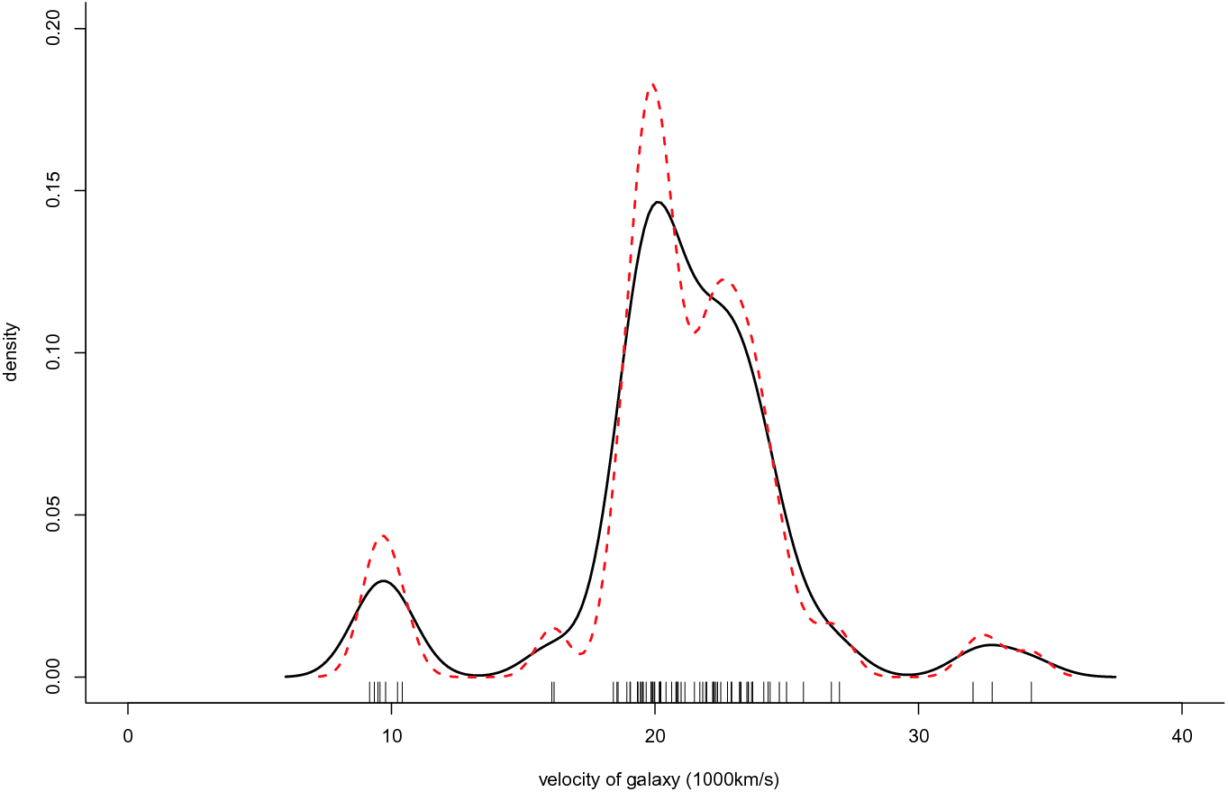
Variable bandwidth and ML estimates for the Galaxies data
4 An Example
As an illustrative example, the Galaxies data of [14] are used. The data represent velocities in km/sec of 82 galaxies from 6 well-separated conic sections of an unfilled survey of the Corona Borealis region. Multimodality in such surveys is evidence for voids and superclusters in the far universe.
 is also verified by the multimodality test of
[6] and thus it is adopted in the present example as well. Figure 1 contains the ML (solid line) and kernel (dashed red line) estimates after scaling the data by 1000. The null hypothesis of goodness-of-fit of the ML estimate was tested at 5% significance level, using as variance the third component of the variance expression. The test procedure gives
is also verified by the multimodality test of
[6] and thus it is adopted in the present example as well. Figure 1 contains the ML (solid line) and kernel (dashed red line) estimates after scaling the data by 1000. The null hypothesis of goodness-of-fit of the ML estimate was tested at 5% significance level, using as variance the third component of the variance expression. The test procedure gives
 and
and  (and one less distinctive at around
  are masked by the ML estimate. On the contrary, the fixed bandwidth estimate
  implemented with the Sheather–Jones bandwidth can detect the change in the pattern of the density. It is worth noting that the variable bandwidth estimate
  has also been tested with the specific data set and found to perform very similarly to
  .
.5 Proof of Theorem 1

 ,
,![$$\begin{aligned} I_3&= \int \left\{ \hat{f}(x; \varvec{\hat{\mu }, \hat{\sigma }, \hat{w}}) - f(x; \varvec{\mu , \sigma , w}) \right\} ^2\,\mathrm{d}x \nonumber \\&= \int \Bigg \{\sum _{i=1}^k \frac{ w_i}{2 \sigma _i^3} \Bigg [ (x- \mu _i)^2 - (x- \hat{\mu }_i)^2 \Bigg ] (1+o_p(n^{-1}))\Bigg \}^2\,\mathrm{d}x = o_p(n^{-1}), \end{aligned}$$](../images/461444_1_En_7_Chapter/461444_1_En_7_Chapter_TeX_Equ12.png)


 from
[10], and
from
[10], and


![$$\begin{aligned} +2 \int \left[ \left\{ \hat{f}(x;h ) - \mathbb E\hat{f}(x; h) \right\} - \left\{ \hat{f}(x; \varvec{\hat{\mu }, \hat{\sigma }, \hat{w}}) - f(x; \varvec{ \mu , \sigma , w}) \right\} \right] \times \end{aligned}$$](../images/461444_1_En_7_Chapter/461444_1_En_7_Chapter_TeX_Equ20.png)


 is a term (see
[5]) such that
is a term (see
[5]) such that
 , this term determines the limiting distribution of the right-hand side of (22). Now, under the null, the fact that
 and by applying the Lyapunov Central Limit Theorem yields
 ,
,  . In this case
 has the same distribution as the first term on the right-hand side of (22). By a direct application of Theorem 1 of
[7] and taking into account also the proof of Theorem 3.2 in
[5], it is straightforward to deduce that
has the same distribution as the first term on the right-hand side of (22). By a direct application of Theorem 1 of
[7] and taking into account also the proof of Theorem 3.2 in
[5], it is straightforward to deduce that
 and hence no term on the right-hand side of (22) dominates the other since both are of the same order. Therefore, in this case, the limiting distribution of
  is given by the sum of the limit distribution of the two terms since, both terms are uncorrelated to each other.