A
More On Data Analysis

Note: You may have learned all you need to know about working with data in Chapter Seven. We have included this appendix for those who need or want to delve more deeply into the subject.

Analyses for Each Level

Different statistics are used to measure central tendency, variability, and analysis of variance depending on the level of data you are dealing with—nominal, ordinal, interval, or ratio. As discussed in Chapter Seven, each level makes certain assumptions about the nature of the data, and these assumptions carry over to the types of statistical analyses appropriate for each.

Measures of Central Tendency

The central tendency is some point at which a data set is split in half. For nominal data that are primarily narrative responses and are often dichotomous variables—yes/no or male/female—the appropriate measure of central tendency (MCT) is the mode. The mode is the most frequently appearing response in the data set.

Ordinal data usually fit on a scale of some sort—such as responses ranging from “strongly agree” to “strongly disagree”—and the MCT is either the median or the mode. The median is the midpoint in the data set or the value at which the data is split exactly in half.

For interval data, which have equal intervals separating each of the values in the response set (1, 2, 3, 4), and ratio data, which contain an absolute zero point, the appropriate MCT may be the mean, median, or mode. The mean is the arithmetic average of the scores in the data set.

Measures of Variability

Two sets of scores might have similar means, medians, or modes but be very different in the scatter of the scores in the data set. There is more variability in one set than the other. Therefore you need a measure that illustrates the spread of these scores. The three most often used measures of variability (MV) are the range, interquartile, and the standard deviation.

For nominal data, the only appropriate MV is the range.

For ordinal data, the MV is the quartile deviation, explained in the following example. Let's say you are collecting data on participant perceptions of a computer literacy training session. The participants are asked to complete an evaluation instrument at the end of the training that asks a variety of questions on the session such as, “Were the objectives met? Was the trainer well prepared? Did the training meet your expectations?” Your instrument includes a Likert scale with these answer choices for each question: strongly agree (5), agree (4), neutral (3), disagree (2), strongly disagree (1).

As the evaluator, you have been asked to analyze each of the questions separately to determine if there is any variability from one question to another. You compile all the responses from 100 participants over the course of four training sessions.

For the question “Was the trainer well prepared?” the responses were strongly agree, 20; agree, 40; neutral, 5; disagree, 20; strongly disagree, 15. You want to calculate the 75th percentile, that is, the score in the range of 1 to 5 where 75 percent of the scores fall below and 25 percent fall above. In this case, of the 100 respondents, 20 of them (20 percent) reported that they strongly agree with this statement. Another 40 (40 percent) indicate that they agree. Thus, the 75th percentile would fall in the agree response category, for a score of 4.

Similarly, calculate the 25th percentile, the score in the range of 1 to 5 where 25 percent of the scores fall below and 75 percent above. In this case, 15 respondents (15 percent) reported that they strongly disagree with this statement. Another 20 (20 percent) indicate that they disagree. Thus, the 25th percentile would fall in the disagree response category, for a score of 2.

Now, to calculate the interquartile deviation, subtract the 25th from the 75th percentile (4 − 2 = 2) and divide that by 2 (2/2 = 1). The interquartile deviation for this distribution of scores is 1.

What this means is that participants’ scores on the question of preparation of the trainer tended to deviate by 1 response category. If you look at the response for this question that was selected by the greatest number of participants (agree = 40 percent), or a response of 4, you can surmise that the majority of all responses fell within plus or minus one point of 4.

Tests of Significance

At some point an evaluator, like a researcher, will want to determine whether a certain treatment—for example, computer-based training—yields better results than another treatment or no treatment. The purpose is to ascertain that the difference in functioning between the two groups has more to do with a specific intervention than with chance. To statistically test this assumption, you can use a variety of tests of significance. For each of these statistical analyses, a number is generated which in turn is compared to an appropriate table of values to determine level of significance.

For nominal data, the most appropriate test is the chi-square (χ²) test. This test relies on data that are in the form of frequency counts (actual counts or percentages that can be converted to frequencies) and on data that have categories (true categories) that are mutually exclusive. This test compares proportions actually observed with those that might be expected. These expected proportions represent one's best guess of what the proportions might look like if all things were equal. They may also be derived from previous experience or studies. The greater the difference between observed and expected results, the greater the chi-square value.

For ordinal data the appropriate test would be a sign test, Wilcoxon signed ranks test, or the Mann-Whitney U test. The sign test and the Wilcoxon could be used if you wanted to determine whether the functioning of individuals in one group at a point prior to treatment (pre) was statistically different from after the treatment (post). If the pre score for a person is higher than the post, then a minus sign (−) is assigned. If pre is the same as post, then a neutral sign (0) is assigned. If the pre score for a person is lower than the post, then a plus (+) sign is attributed. Consequently, it becomes the preponderance of one sign over the others that determines significance. Similarly, if you wish to determine whether the difference between the scores of individuals in two different groups is statistically significant, you could use the Mann-Whitney U test. In all three tests the pre and post scores, or the group 1 and group 2 scores, are compared and the differences (sign) are noted. All three tests and others are described in Seigel (1956).

For interval and ratio data, the appropriate test would be a t test. This test determines whether the means of two different groups are significantly different given a preselected probability level. The dependent t test would be used if you wanted to determine whether the functioning of individuals in one group from a point prior to treatment (pre) was statistically different from their functioning after the treatment (post). In this test the mean is calculated for the entire data set. Then each score is subtracted from the mean. These differences are squared and added together (sum of squares). Then the data are used in a formula to determine the t value. This value is compared to a t-test table to determine significance.

You would use a different test, the independent t test, if you wished to determine whether the difference between the scores of individuals in two different groups was statistically significant.

Correlations

At some point in an evaluation you may wish to assess to what degree a relationship exists between two or more variables. This does not infer a causal relationship as in the tests of significance, just a relationship. The degree of relationship is calculated as a correlation coefficient and measured on a scale between −1.00 and +1.00. If two variables are highly correlated, you will see a correlation coefficient that is closer to 1.00 (− or +) than to zero. If there is a weak correlation, the correlation coefficient will be closer to zero.

For ordinal data the appropriate correlation would be the Spearman rho. In this statistic, an inference is made that the data sets are rank ordered—for example, seniority at the time of training.

For interval and ratio data, the appropriate correlation would be the Pearson r. Like other measures at these data levels, the Pearson r uses each score in both distributions.

Significance Testing

One of the most powerful tools that evaluators and researchers have is the ability to infer causality by analyzing data. As discussed in Chapter Eight, the more rigorous the study and the more quantitative the data, the more you can employ formulas of statistical significance that will allow you to draw such inferences. To many people, the basic assumptions underlying significance testing are so difficult to grasp that they simply “take your word for it” and press their “I believe” button when using tests of statistical significance or reading the results. However, an understanding of the procedures will explain what the tests can really do and what they mean, so we will take a look at them.

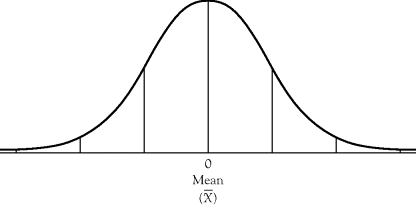
Let's begin by talking about the normal curve. If you were to gather a set of scores and calculate the mean for those scores, you would assume that the scores below the mean and those above the mean would be evenly distributed. In other words, there would be a similar number of scores above and below the mean, as illustrated in Figure A.1.

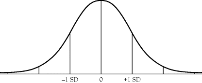
The second assumption, given what you have learned about the standard deviation, would be that 34 percent of the scores in the set fall on the minus side of the mean and 34 percent fall on the positive side of the mean. Or a total of 68 percent of the scores in the set should fall one standard deviation (SD) about the mean, as illustrated in Figure A.2.

Figure A.2 Normal Curve and One Standard Deviation

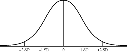
Third, if you were to go out from the mean a second standard deviation, you could now account for an additional 13.5 percent of the scores on the minus side and 13.5 percent on the positive side of the mean. Thus, if you looked two standard deviations about the mean, you should account for 95 percent of the scores, as illustrated in Figure A.3.

Figure A.3 Normal Curve and Two Standard Deviations

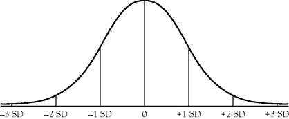
If you were to extend one more standard deviation you should account for 2 percent of the scores on either side of the mean, or an additional 4 percent, for a total of 99 percent of the scores, as illustrated in Figure A.4.

Figure A.4 Normal Curve and Three Standard Deviations

Beyond three standard deviations you would be accounting for the remaining variance (0.05 percent below and 0.05 percent above the mean). The important point is the totals we have discussed: one standard deviation should account for 68 percent of the scores; two standard deviations should account for 95 percent of the scores, and three standard deviations should account for 99 percent of the scores. Statistical significance lies beyond the third deviation.

If the set of scores you possess is normally distributed, then the aforementioned proportions should hold. Put another way, if left purely to chance, the scores in your set should fall as we have described. If they do, there really is nothing remarkable or statistically significant about your set of scores.

However, if your distribution does not follow this pattern and many more scores fall into the range defined by four or even five standard deviations, then you have a distribution that is somewhat remarkable. Why? If your assumption is that 99 percent of the scores should fall within the four standard deviations about the mean, but many more than 0.05 percent fall in the fourth standard deviation range, then your distribution could not have been expected to occur simply by chance. Instead, the assumption is that something happened to cause those scores to fall outside of the expected distribution. This something, you would like to believe, was your program. This is where we get the 0.05 level of significance that is used to designate those findings of statistical analyses that are deemed statistically significant, or beyond chance occurrence.

This level of significance is constant regardless of the type of statistical analysis—whether t test, correlation coefficients, or Wilcoxon test—and denotes a level of confidence that your findings were attributable to something more than chance. In some research a higher level of confidence is desirable, so the determination of significance is taken beyond the .05 level to the .01 or .001 levels, examining frequency even farther from the mean, to five or six standard deviations. However, the .05 level of significance is sufficient for most evaluation and research purposes.

Statistical and Practical Significance

Usually in an evaluation you have neither the need nor the luxury to perform complex statistical analyses. If you can do so, it will contribute a great deal to the believability of your findings. Granted, you were appointed or hired because of your expertise and knowledge about the process, but having the “hard facts and figures” to back your anecdotal information and impressions gives your conclusions considerably more credibility.

You do not necessarily have to be dismayed if in conducting a test of significance on your data set you find no statistically significant findings. At times there can be only practical significance to your findings. Take the example in Chapter Two of the evaluation of a high school career development program. In this program the participating students attended academic classes three days of the school week and were given structured activities on job sites the other two days. At the close of the school year, participating and nonparticipating students were administered a standardized achievement examination. When the results were compared, there were no statistically significant differences between the posttest scores of the treatment and the control groups. In fact, the means of the two distributions were quite similar. At first glance one would be inclined to conclude that this Career Education Program was a failure. However, these career education students were in academic classes for only three days per week compared to the five days of the control students, a difference with significant implications for any evaluation. Yet they still achieved an equal level academically and also benefited from a wealth of work site experiences. Perhaps the Career Education Program did not help these students score higher academically, but it certainly didn't hurt them as they pursued their work-study agenda.

For more references on statistical analysis and for related software, see the Further Reading and Software lists at the end of Chapter Seven.