4.1 Introduction
Because of poor channel conditions, correct reception at a certain target data rate can sometimes become impossible. Therefore, packet retransmission protocols are used in modern wireless communications systems to improve the reliability of data transmission. Specifically, when a one-bit feedback link is available from the receiver to the transmitter, the simple scheme of hybrid automatic repeat request (ARQ) with Chase combining (HARQ-CC) can be employed, where the same packet is retransmitted in the event of decoding failure.
In this chapter, we would like to address the design of hybrid RF-baseband precoding and combining suitable for massive multiple-input multiple-output (MIMO) with hybrid ARQ. In particular, based on the perfect channel state information (CSI), we consider a progressive approach to the hybrid precoder and combiner design in an attempt to exploit the temporal diversity inherent in packet retransmissions. Conditioned on the knowledge of previous retransmissions, the hybrid precoder and combiner are sequentially optimized for the current ARQ round without considering potential future retransmissions. To this end, we propose a two-step strategy to optimize the hybrid RF-baseband precoders/combiners with the objective of maximizing the spectral efficiency. On the heuristic assumption that the linear minimum mean square error (MMSE) filter is perfectly realizable by the two-stage receive combiner, we separate the derivation of the hybrid precoding from the hybrid combining. At the transmitter, during each ARQ round, we choose the RF precoder either from the set of transmit array response vectors or from a discrete Fourier transform (DFT)-based codebook. Built upon the selected RF precoder, the optimal beamformer at baseband is analytically shown to be a function of the generalized eigenvectors of the effective channel and RF precoder for the current ARQ retransmission, while the transmit power is allocated based on the precoding solutions from the previous and current packet retransmissions. At the receiver, a novel hybrid combining structure is proposed to address the issue of increased computational and storage complexity caused by repeated packet retransmissions. To minimize the performance loss of the decoupled precoding-combining optimization, the two-step strategy is further applied to derive the hybrid combining solution as an approximation of the optimal linear digital counterpart in terms of error performance. Through numerical simulations, we validate the efficacy of the proposed progressive approach to hybrid precoding and combining from (1) its comparable performance with the fully digital optimal progressive scheme, and (2) its performance advantage over other hybrid baseline that is oblivious to the presence of time diversity.
Although previous works, e.g., [1–3], have proposed various solution techniques for hybrid precoding and combining in the context of massive MIMO, they do not directly carry over when hybrid ARQ is incorporated. The study in this chapter is motivated by the observation that sequential precoding optimization is unique to ARQ systems as data retransmission occurs only if the previous transmissions fail. Since it is not possible to alter the previous transmission attempts of a data packet and another retransmission attempt may not be required after the current transmission, the transmitter can only optimize the current transmission for each ARQ round with respect to the desired performance metric. In theory, the formulation of matrix reconstruction as in Chap. 3 can be exploited to solve for the hybrid design as an approximation of the optimal solution. This nonetheless requires the knowledge of the fully digital solutions, which is generally nontrivial to obtain in the first place. Furthermore, such an approach tends to lead to suboptimal power loading schemes at baseband. In contrast, the proposed progressive precoding solution takes into account power allocation for each round of packet retransmission, and also gives insights into the relation between the precoder for the current ARQ transmission and the previous ones. Mathematically, the presence of the RF stage in the power constraint also necessitates a different solution approach.
The rest of this chapter is organized as follows. In Sect. 4.2, we describe the system model of massive MIMO with hybrid ARQ where hybrid precoding and combining are employed. We develop the proposed methods of progressive optimization of hybrid precoding and combining in Sects. 4.3 and 4.4, respectively. Illustrative results are provided in Sect. 4.5, where the proposed progressive hybrid solution is numerically compared with various baselines. Concluding remarks are made in Sect. 4.6.
4.2 System Model and Problem Statement
 denote the number of data streams to be transmitted. As a result of a limited number of RF chains, a hybrid RF-baseband precoder/combiner in place of a single-stage, fully digital precoder/combiner is employed. As illustrated in Fig. 4.1, the data streams are first linearly transformed using a low-dimensional baseband precoder
  , the output of which is then precoded by a high-dimensional RF precoder
  . The RF precoder is assumed to be implemented using analog phase-shifters, i.e., the elements are constrained to satisfy
 ![$$\vert [{\mathbf {F}}_{\mathrm {RF}}]_{i,j}\vert =\frac {1}{\sqrt {N_{\mathrm {t}}}},1\leq i\leq N_{\mathrm {t}},1\leq j\leq n_{\mathrm {t}}$$](../images/470489_1_En_4_Chapter/470489_1_En_4_Chapter_TeX_IEq4.png) .
.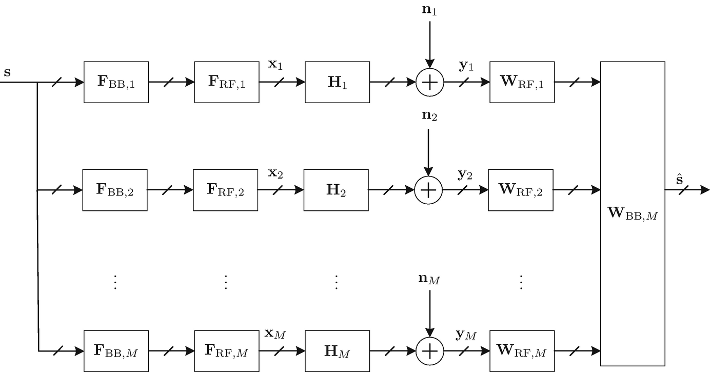
Hybrid RF-baseband precoding and combining for M rounds of packet retransmission in a point-to-point massive MIMO hybrid ARQ system

 ,
,  denotes the massive MIMO channel between the transmitter and receiver during the mth retransmission of the data vector s, and is assumed to change independently from transmission to transmission, and
  is the spatially white Gaussian noise with variance
  . In particular, we characterize H
m, ∀m by a parametric clustered channel model [1, 4], in which the channel matrix is a sum of contributions of N
cl scattering clusters, each with N
ray propagation paths. Assuming uniform linear arrays (ULA) at both link ends, the MIMO channel is generically expressed as1
. In particular, we characterize H
m, ∀m by a parametric clustered channel model [1, 4], in which the channel matrix is a sum of contributions of N
cl scattering clusters, each with N
ray propagation paths. Assuming uniform linear arrays (ULA) at both link ends, the MIMO channel is generically expressed as1 
 is a normalization factor such that
 ![$$\mathbb {E}[\left \Vert \mathbf {H}\right \Vert _{\mathrm {F}}^{2}]=N_{\mathrm {r}}N_{\mathrm {t}}$$](../images/470489_1_En_4_Chapter/470489_1_En_4_Chapter_TeX_IEq10.png) , and
, and  is the i.i.d. complex path gain of the lth ray in the ith scattering cluster. The vector
  (
( ) represents the normalized receive (transmit) array response vector at an azimuth angle of arrival (AoA)
  (angle of departure (AoD)
  ). For a generic N-element ULA on the y-axis, the array response is expressed as [1]
 ![$$\displaystyle \begin{aligned} {\mathbf{a}}_{\mathrm{ULA}}\left(\phi\right)=\frac{1}{\sqrt{N}}\left[1,\,e^{\jmath2\pi d_{\lambda}\sin\left(\phi\right)},\cdots,\,e^{\jmath\left(N-1\right)2\pi d_{\lambda}\sin\left(\phi\right)}\right]^{\mathrm{T}},{} \end{aligned} $$](../images/470489_1_En_4_Chapter/470489_1_En_4_Chapter_TeX_Equ1.png)
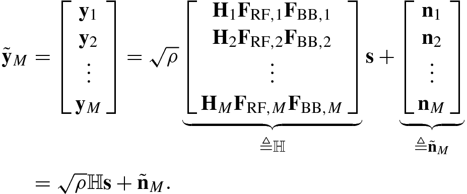
![$${\mathbf {R}}_{\tilde {n}}\triangleq \mathbb {E}[\tilde {\mathbf {n}}_{M}\tilde {\mathbf {n}}_{M}^{\mathrm {H}}]=\sigma _{n}^{2}{\mathbf {I}}_{MN_{\mathrm {r}}}$$](../images/470489_1_En_4_Chapter/470489_1_En_4_Chapter_TeX_IEq19.png) . The fact that the same signal is transmitted in the event of decoding failure enables the coherent combining of all the received signals across different ARQ rounds. Ideally, the combining should take place in both the RF and baseband domains for the optimal performance, which would require storage of the high-dimensional received signals
. The fact that the same signal is transmitted in the event of decoding failure enables the coherent combining of all the received signals across different ARQ rounds. Ideally, the combining should take place in both the RF and baseband domains for the optimal performance, which would require storage of the high-dimensional received signals  from all ARQ rounds and applying to the aggregate received signal
  an RF combiner of size MN
r × Mn
r followed by a baseband combiner of size Mn
r × N
s. Unfortunately, these high-dimensional combiners pose nontrivial computational and storage complexity, especially when N
r is large. Furthermore, additional RF phase-shifters are needed to implement the joint combining in the RF domain.3 Out of these concerns, in this work, we propose to first perform independent RF combining of the received signals from each ARQ round, and then perform joint baseband combining of the RF-processed received signals across all ARQ rounds, as illustrated in Fig. 4.1. Accordingly, after the Mth ARQ round, the signal at the output of the hybrid combiner can be written as
an RF combiner of size MN
r × Mn
r followed by a baseband combiner of size Mn
r × N
s. Unfortunately, these high-dimensional combiners pose nontrivial computational and storage complexity, especially when N
r is large. Furthermore, additional RF phase-shifters are needed to implement the joint combining in the RF domain.3 Out of these concerns, in this work, we propose to first perform independent RF combining of the received signals from each ARQ round, and then perform joint baseband combining of the RF-processed received signals across all ARQ rounds, as illustrated in Fig. 4.1. Accordingly, after the Mth ARQ round, the signal at the output of the hybrid combiner can be written as 
 is the aggregate RF combiner with the mth component
  1 ≤ m ≤ M, as the RF combiner with respect to the received signal y
m, and
1 ≤ m ≤ M, as the RF combiner with respect to the received signal y
m, and  is a baseband combiner used during the Mth ARQ round. The achievable rate per channel use, i.e., spectral efficiency, with the proposed precoding and combining strategy after M ARQ rounds is therefore expressed as
 and
and  for notational simplicity.
4.3 Progressive Hybrid Precoding Design
In this section, we formulate the progressive hybrid precoding problem during the Mth ARQ round of data retransmission. Built upon the hybrid precoders  and hybrid combiners
  used for the previous retransmission attempts, the objective is to find the hybrid precoder {F
RF,M, F
BB,M} and hybrid combiner {W
RF,M, W
BB,M} during the Mth ARQ round such that
used for the previous retransmission attempts, the objective is to find the hybrid precoder {F
RF,M, F
BB,M} and hybrid combiner {W
RF,M, W
BB,M} during the Mth ARQ round such that  in (4.2) is maximized.
 in (4.2) is reduced to the mutual information between s and
  , i.e.,
  , as given by
 . The problem of interest is accordingly formulated as
 , we propose a two-step solution technique. In the first step, we choose the RF precoder F
RF,M to be one of the feasible solutions from the set
, we propose a two-step solution technique. In the first step, we choose the RF precoder F
RF,M to be one of the feasible solutions from the set  , say G
RF,M, and conditioned on this choice, we derive the closed-form solution for the optimal baseband precoder
, say G
RF,M, and conditioned on this choice, we derive the closed-form solution for the optimal baseband precoder  . This procedure is repeated for each feasible G
RF,M to generate a set of
. This procedure is repeated for each feasible G
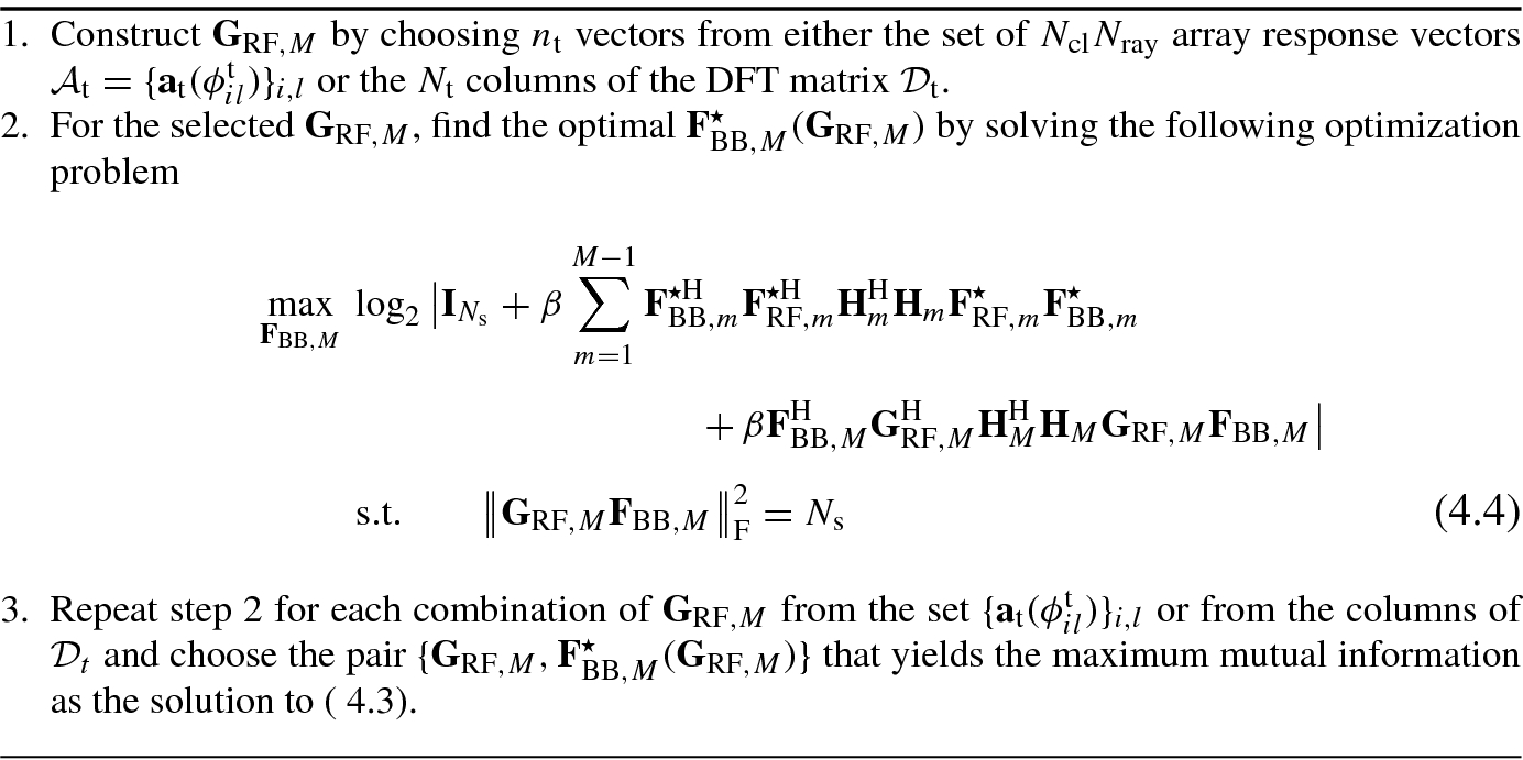
RF,M to generate a set of  , from which the pair that yields the maximum mutual information in (4.3) is declared as the solution to the original problem. We remark that unlike the one-shot approach based on matrix reconstruction in [1], the proposed two-step technique obviates the need for knowing the fully digital solution, and enjoys the flexibility of performing waterfilling-based power loading at baseband.
Clearly, the set of constant-modulus RF precoders  contains an unlimited number of elements. To facilitate the RF precoding optimization, we consider two suboptimal but effective alternatives, where the columns of the RF precoder F
RF,M are assumed to be chosen either from the set of N
cl
N
ray transmit array response vectors
contains an unlimited number of elements. To facilitate the RF precoding optimization, we consider two suboptimal but effective alternatives, where the columns of the RF precoder F
RF,M are assumed to be chosen either from the set of N
cl
N
ray transmit array response vectors  [1] or from the N
t columns of the N
t-dimensional DFT matrix
[1] or from the N
t columns of the N
t-dimensional DFT matrix ![$$\mathcal {D}_{\mathrm {t}}\triangleq \left [\frac {1}{\sqrt {N_{\mathrm {t}}}}e^{-\frac {\jmath 2\pi mn}{N_{\mathrm {t}}}}\right ],0\leq m,n\leq N_{\mathrm {t}}-1$$](../images/470489_1_En_4_Chapter/470489_1_En_4_Chapter_TeX_IEq40.png) [2]. The rationale for constraining the columns of the RF precoder to the finite sets
[2]. The rationale for constraining the columns of the RF precoder to the finite sets  and
and  for the ARQ retransmission is threefold: (1) on one hand, the optimal progressive digital precoder has been known to be a function of a unitary matrix whose columns span the row space of the channel H
M [7]. On the other hand, it has been observed in [1] that under certain conditions, the set of transmit array response vectors
for the ARQ retransmission is threefold: (1) on one hand, the optimal progressive digital precoder has been known to be a function of a unitary matrix whose columns span the row space of the channel H
M [7]. On the other hand, it has been observed in [1] that under certain conditions, the set of transmit array response vectors  serves as another basis for the row space of the channel H
M; (2) as indicated by the definition (4.1), the transmit array response vector
serves as another basis for the row space of the channel H
M; (2) as indicated by the definition (4.1), the transmit array response vector  , consists of constant-modulus entries; (3) when angle-domain quantization is considered as an option to reduce the overhead of estimating the complete AoD information, the array response vector-based RF precoding design can still be directly applied. One extreme case is the DFT-based codebook, which represents blind uniform quantization of the azimuth AoDs. Interestingly, in the large-scale array regime, the DFT matrix becomes an asymptotically good approximation for the channel eigen-space [8]. Our proposed approach to generate the hybrid RF-baseband precoder for the Mth ARQ retransmission is summarized in Algorithm 1.
Algorithm 1 Two-step progressive hybrid RF-baseband precoding design
 to (4.4), we observe that given the eigenvalue decomposition

 , and
, and  . On the other hand, following the orthonormality of U, the power constraint in (4.4) is equivalent to
  . In other words, we can reformulate the problem (4.4) as
Theorem 4.1
 and
and
 as
as

 Let
Let  denote the indices of the largest N
s elements of the set
denote the indices of the largest N
s elements of the set  such that
  . Denote
  Let P
1,M and P
2,M be the permutation matrices such that the diagonal elements of
Let P
1,M and P
2,M be the permutation matrices such that the diagonal elements of  are in non-decreasing order while those of
  are in non-increasing order. Then the optimal solution to (4.5) is given by
 with
with

and c chosen such that  , and S
M selects the N
s columns of A
M indexed by
, and S
M selects the N
s columns of A
M indexed by  .
.
Proof
See Appendix 1.
Remark 4.1
- 1.
The optimal beamforming subspace is spanned by the generalized eigenvectors A M of the Gram matrices of the effective channel H M G RF,M and the RF precoder G RF,M.
- 2.
The optimal beamforming directions are determined by the selection matrix S M, which picks the N s largest indices of the set
 .
. - 3.
The diagonal matrix
 implements the waterfilling-based power loading.
 - 4.
The permutation matrices P 1,M and P 2,M achieve the optimal reverse pairing of the singular values of the previous precoded transmissions
 with the largest N
s elements of the set
with the largest N
s elements of the set  related to the current transmission.
 - 5.
For the initial transmission, i.e., M = 1, the permutation matrices become an identity matrix, i.e.,
 , and the transmit power is loaded according to
  , 1 ≤ j ≤ N
s.
, 1 ≤ j ≤ N
s.
4.4 Progressive Hybrid Combining Design
In the previous section, by heuristically assuming that the fully digital linear MMSE combiner can be perfectly reconstructed by the hybrid RF-baseband counterpart, we were able to abstract the hybrid combining effect on the achievable rate, and decouple the precoding from the combining optimization. In the existing works such as [1], the reconstruction was addressed in terms of the combining structure, and was formulated as a matrix reconstruction problem. In doing this, the fully digital solution needs to be known. However, as discussed in Sect. 3.2, such knowledge might not be practically obtainable in light of the storage requirement imposed by the high-dimensional received signals across multiple ARQ rounds. Furthermore, since the matrix reconstruction formulation attempts to generate the RF and baseband combiners simultaneously, suboptimal baseband solutions are likely to result. In view of these drawbacks, we consider applying the two-step approach from the previous section to the hybrid combining design in this section.
 generated from the procedure developed in Sect. 4.3 and the RF combiners
  , the idea is to design the hybrid RF-baseband combiner for the current ARQ round, i.e., {W
RF,M, W
BB,M}, as a good approximation of the fully digital solution in terms of error performance. To this end, we consider the minimization of MSE between the transmitted signal and the aggregate received signals, which leads to the problem formulation as
, the idea is to design the hybrid RF-baseband combiner for the current ARQ round, i.e., {W
RF,M, W
BB,M}, as a good approximation of the fully digital solution in terms of error performance. To this end, we consider the minimization of MSE between the transmitted signal and the aggregate received signals, which leads to the problem formulation as ![$$\displaystyle \begin{aligned} \begin{array}{rcl} &\displaystyle \underset{{\scriptstyle {\mathbf{W}}_{\mathrm{RF},M},{\mathbf{W}}_{\mathrm{BB},M}}}{\min} &\displaystyle \mathbb{E}\left[\left\Vert \mathbf{s}-{\mathbf{W}}_{\mathrm{BB},M}^{\mathrm{H}}\mathbb{W}_{\mathrm{RF},M}^{\mathrm{H}}\tilde{\mathbf{y}}_{M}\right\Vert _{2}^{2}\right] \\ &\displaystyle \mathrm{s.t.} &\displaystyle {\mathbf{W}}_{\mathrm{RF},M}\in\mathcal{W}_{RF},{} \end{array} \end{aligned} $$](../images/470489_1_En_4_Chapter/470489_1_En_4_Chapter_TeX_Equ5.png)
 denotes the set of feasible RF combiners with constant-modulus elements. It is straightforward to show that the objective in (4.6), denoted as
  , can be evaluated as
 ![$$\displaystyle \begin{aligned} \mathcal{E} & =1+\sigma_{n}^{2}\mathrm{tr}\left[{\mathbf{W}}_{\mathrm{BB},M}^{\mathrm{H}}\mathbb{W}_{\mathrm{RF},M}^{\mathrm{H}}\left(\beta\mathbb{H}\mathbb{H}^{\mathrm{H}}+{\mathbf{I}}_{MN_{\mathrm{r}}}\right)\mathbb{W}_{\mathrm{RF},M}{\mathbf{W}}_{\mathrm{BB},M}\right] \\ & \quad -2\frac{\sqrt{\rho}}{N_{\mathrm{s}}}\Re\left\{ \mathrm{tr}\left(\mathbb{H}^{\mathrm{H}}\mathbb{W}_{\mathrm{RF},M}{\mathbf{W}}_{\mathrm{BB},M}\right)\right\} .{} \end{aligned} $$](../images/470489_1_En_4_Chapter/470489_1_En_4_Chapter_TeX_Equ6.png)
 , say B
RF,M, and then conditioned on the RF combiner B
RF,M, computes the optimal baseband combiner
, say B
RF,M, and then conditioned on the RF combiner B
RF,M, computes the optimal baseband combiner  . This procedure is repeated to generate a pair
  for each chosen
  , where the MMSE-achieving pair is treated as the solution to the original problem. By solving the first-order derivative of (4.7), i.e.,
 , as a function of the RF combiner, can be expressed in a closed form as
 ![$$\displaystyle \begin{aligned} {\mathbf{W}}_{\mathrm{BB},M}^{\star}\left({\mathbf{W}}_{\mathrm{RF},M}\right)=\frac{\sqrt{\rho}}{N_{\mathrm{s}}\sigma_{n}^{2}}\left[\mathbb{W}_{\mathrm{RF},M}^{\mathrm{H}}\left(\beta\mathbb{H}\mathbb{H}^{\mathrm{H}}+{\mathbf{I}}_{MN_{\mathrm{r}}}\right)\mathbb{W}_{\mathrm{RF},M}\right]^{-1}\mathbb{W}_{\mathrm{RF},M}^{\mathrm{H}}\mathbb{H}.{} \end{aligned} $$](../images/470489_1_En_4_Chapter/470489_1_En_4_Chapter_TeX_Equ7.png)
 to either the finite set of N
cl
N
ray receive array response vectors
to either the finite set of N
cl
N
ray receive array response vectors  [1] or the N
r columns of the N
r-dimensional DFT matrix
[1] or the N
r columns of the N
r-dimensional DFT matrix ![$$\mathcal {D}_{\mathrm {r}}=\left [\frac {1}{\sqrt {N_{\mathrm {r}}}}e^{-\frac {\jmath 2\pi mn}{N_{\mathrm {r}}}}\right ],0\leq m,n\leq N_{\mathrm {r}}-1$$](../images/470489_1_En_4_Chapter/470489_1_En_4_Chapter_TeX_IEq78.png) . We formally summarize the proposed strategy for MMSE hybrid combining for the Mth ARQ round as follows.
. We formally summarize the proposed strategy for MMSE hybrid combining for the Mth ARQ round as follows.Algorithm 2 Two-step progressive hybrid RF-baseband combining design
- 1.
Construct B RF,M and accordingly
 by choosing n
r vectors from either the set of N
cl
N
ray receive array response vectors
by choosing n
r vectors from either the set of N
cl
N
ray receive array response vectors  or the N
r columns of the DFT matrix
or the N
r columns of the DFT matrix  .
. - 2.
For the selected B RF,M, compute the MMSE baseband combiner based on (4.8) and the MSE for the pair
 based on (4.7).
 - 3.
Repeat step 2 for each combination of B RF,M from
 or from the columns of
  , and choose the pair
  from step 2 that minimizes the MSE as the solution to (4.6).
4.5 Illustrative Results and Discussions
In this section, we present illustrative results comparing the performance of various precoding and combing methods for massive MIMO systems with packet retransmissions. The channel model is realized assuming N
cl = 5 scattering clusters with N
ray = 2 rays per cluster. We assume ULAs with directional antennas at the transmitter and omni-directional antennas at the receiver. The antenna elements are critically spaced, i.e., d
λ = 0.5. For each cluster, the mean azimuth AoD is assumed to be uniformly distributed over a 60∘ sector angle, i.e.,  , whereas the mean azimuth AoA at the receiver is uniformly distributed over
  . The azimuth AoA and AoD of each ray are Laplacian distributed with angle spread of 7.5∘. We assess the two proposed schemes of progressive hybrid precoding and combining (PHPC): (1) the columns of the RF precoder and combiner are chosen from the set of array response vectors, as denoted by PHPC-AR; (2) the columns of the RF precoder and combiner are chosen from those of the DFT matrices, as denoted by PHPC-DFT. The performance of PHPC is numerically evaluated in terms of achievable rates and MSE. In the former case, we present for comparison the optimal progressive digital precoding (OPDP) scheme of [7], where an ML receiver was employed. Hence, the rate performance of such a design can be treated as a benchmark for any other precoding and combining scheme. In the latter case, we plot for comparison the OPDP scheme of [9] which addressed the minimization of MSE. The sparse precoding and combining (SPC) approach of [1] serves as another baseline. We note that SPC [1] does not take into account packet retransmissions, and it cannot be straightforwardly extended to systems equipped with packet retransmission. This is because the premise of matrix approximation that the idea of SPC was built upon would no longer hold if the previous retransmission attempts were incorporated. Hence, we adapt SPC [1] to the case of ARQ by designing the sparse precoder and combiner for each ARQ round independently. In doing this, we may gain some insights into when the use of time diversity in the precoding/combining design would become advantageous. In view of the limited scattering in the environment, only a small number of data streams is assumed to be transmitted. All the results presented here are averaged over 1000 random realizations of the massive MIMO channel.
4.5.1 Small M
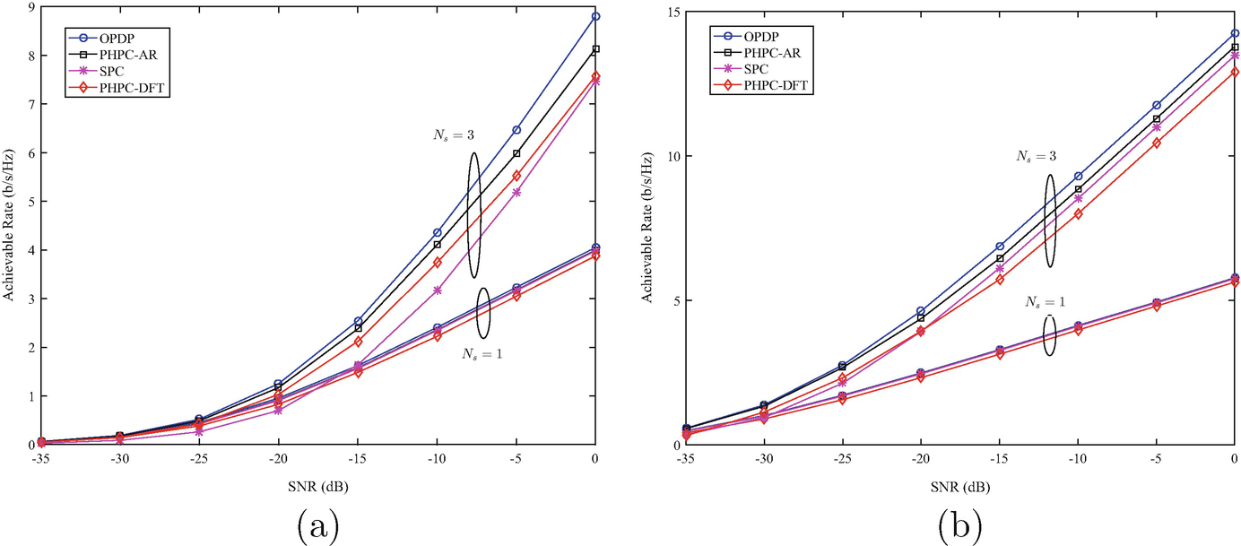
Achievable rates of various ARQ precoding and combining schemes with n t = n r = 3, M = 2, and angle spread of 7.5°. (a) N t = 32, N r = 8. (b) N t = 128, N r = 32
4.5.2 Large M
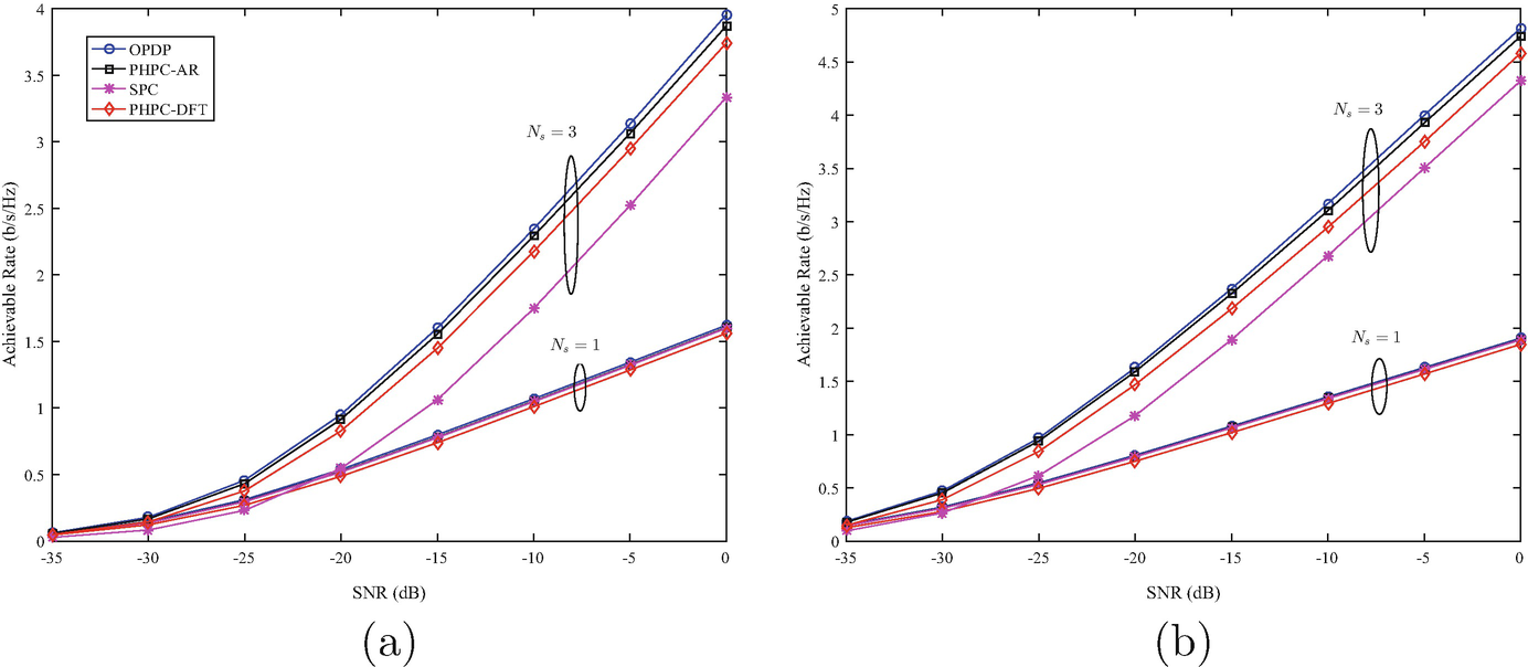
Achievable rates of various ARQ precoding and combining schemes with n t = n r = 3, M = 6, and angle spread of 7.5°. (a) N t = 32, N r = 8. (b) N t = 64, N r = 16
4.5.3 Increasing Number of RF Chains
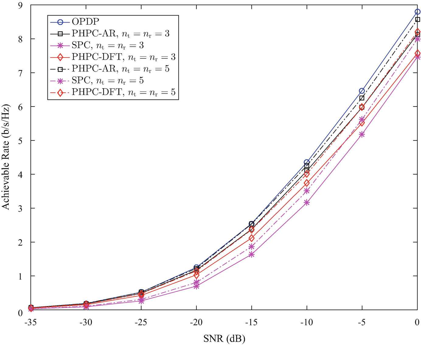
Achievable rates of various ARQ precoding and combining schemes with different number of RF chains at the transmitter and receiver for N t = 32, N r = 8, M = 2, N s = 3, and angle spread of 7.5°
4.5.4 Impact of Angle Spread

Achievable rates versus azimuth angle spread at the transmitter and receiver for N s = 2, n t = n r = 2. (a) M = 2. (b) M = 6
4.5.5 Quantization of RF Precoder/Combiner
 and
and  , respectively. In practice, such knowledge of the exact AoDs
  and AoAs
  of all the scattering paths might not always be readily available. For example, some paths might not be spatially resolvable as a result of the finite dimension of the antenna array [10]. However, the AoD/AoA support can be inferred through estimating the mean AoD/AoA and angle spread. Suppose that the azimuth AoDs and AoAs lie within
  and
and  , respectively. One potential approach to alleviating the channel estimation overhead is to employ uniform quantization of the azimuth angular space such that the array response vectors for F
RF,M and W
RF,M during the Mth ARQ round are generated from the set of angles
, respectively. One potential approach to alleviating the channel estimation overhead is to employ uniform quantization of the azimuth angular space such that the array response vectors for F
RF,M and W
RF,M during the Mth ARQ round are generated from the set of angles 
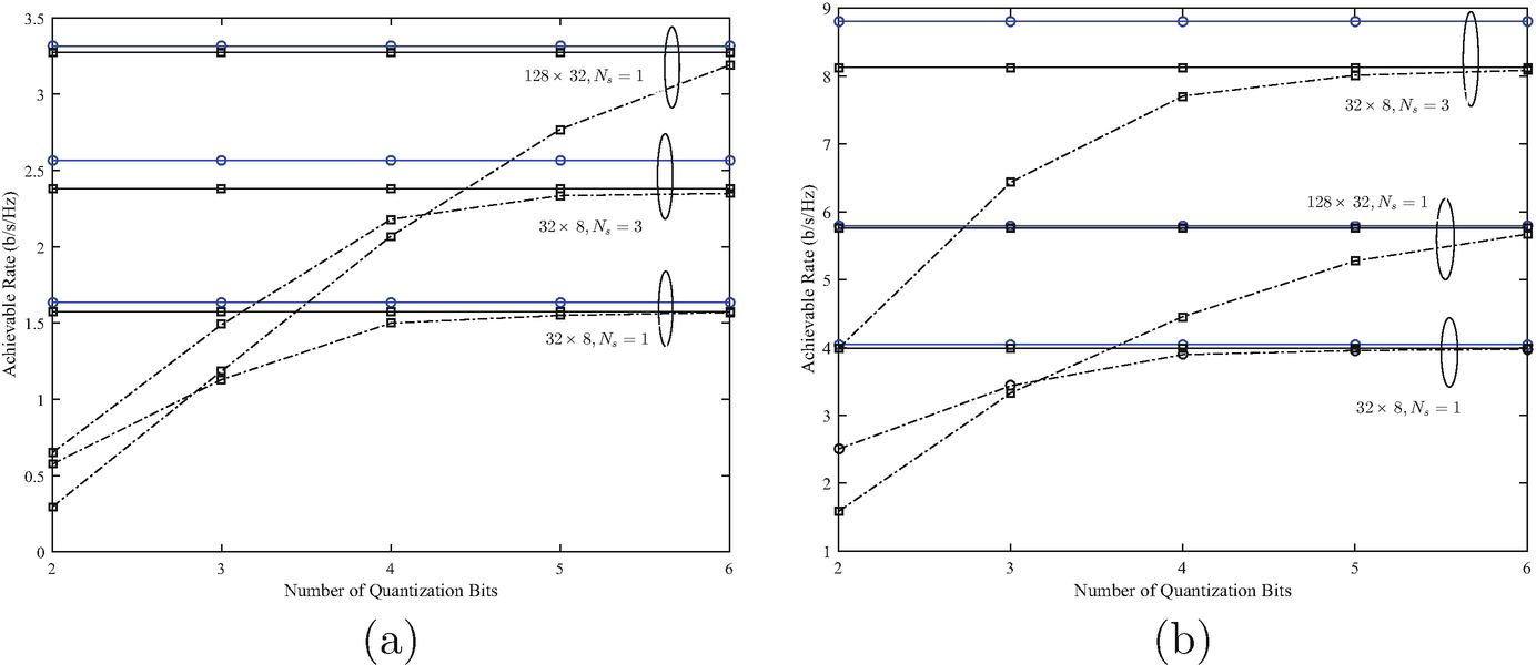
Achievable rates versus the number of quantization bits  for the azimuth AoD and AoA at the transmitter and receiver with n
t = n
r = 3, M = 2, and azimuth angle spread of 7.5°. (a) SNR = −15 dB. (b) SNR = 0 dB
for the azimuth AoD and AoA at the transmitter and receiver with n
t = n
r = 3, M = 2, and azimuth angle spread of 7.5°. (a) SNR = −15 dB. (b) SNR = 0 dB
For a larger antenna array configuration of N t = 128, N r = 32, even for single-stream beamforming, we would need 6 bits for quantization to deliver a comparable performance with the perfect CSI case. Since there is a trade-off between the number of quantization bits to achieve a better performance and the number of combinations to be searched to generate the RF precoder/combiner, we see that N ϕ = 5 can be a suitable choice.
4.5.6 MSE

MSE performance of various ARQ precoding and combining schemes with n t = n r = 3, and angle spread of 7.5°. (a) N s = 1. (b) N s = 3
4.5.7 Complexity
 and
and  combinations from the set of array response vectors
  and
and  , respectively. In the case of PHCP-DFT where the feasible sets of the RF precoder and combiner are constrained to the columns of N
t-dimensional and N
r-dimensional DFT matrices, respectively, the number of possibilities to be evaluated is
, respectively. In the case of PHCP-DFT where the feasible sets of the RF precoder and combiner are constrained to the columns of N
t-dimensional and N
r-dimensional DFT matrices, respectively, the number of possibilities to be evaluated is  for the RF precoding and
  for the RF combining. If the values of N
cl, N
ray, N
t and N
r are very large, finding the solution using PHPC-AR and PHCP-DFT in real-time may not be practical. On the contrary, the quantization approach examined in Sect. 4.5.5 requires the evaluation of
for the RF combining. If the values of N
cl, N
ray, N
t and N
r are very large, finding the solution using PHPC-AR and PHCP-DFT in real-time may not be practical. On the contrary, the quantization approach examined in Sect. 4.5.5 requires the evaluation of  and
and  combinations for the RF optimization at the transmitter and receiver, respectively, which are independent of the number of antennas and the number of scattering paths in the propagation environment. Using PHCP-AR and PHCP-DFT as benchmarks, one can consider the use of reduced-complexity heuristic search algorithms such as the Tabu search [11] to generate the RF solutions in real time. Once the RF precoder and combiner are found, the closed-form baseband precoder and combiner can be computed with the number of flops on the order of
  and
and  , respectively. This is a significant decrease in the computational complexity compared with the optimal solution OPDP, which requires
  flops in the derivation of the fully digital precoder and worse-case receiver complexity scaled exponentially with N
r. For the case of SPC, it takes
flops in the derivation of the fully digital precoder and worse-case receiver complexity scaled exponentially with N
r. For the case of SPC, it takes  flops to generate the hybrid precoding solution and
  flops to generate the hybrid combining solution. For a more intuitive comparison, we list in Table 4.1 the number of real flops per ARQ round required by the dominant operations of the presented precoding and combining schemes. We focus on the case of N
s = 3 data streams and M = 6 ARQ rounds of retransmission for both the small and large antenna configurations.
flops to generate the hybrid combining solution. For a more intuitive comparison, we list in Table 4.1 the number of real flops per ARQ round required by the dominant operations of the presented precoding and combining schemes. We focus on the case of N
s = 3 data streams and M = 6 ARQ rounds of retransmission for both the small and large antenna configurations. Comparison of computational complexity (real flops)
Real flops (in million) | ||||
|---|---|---|---|---|
Antenna configuration | OPDP | PHPC-AR | PHPC-DFT | SPC |
N t = 32, N r = 8 | 0.43 | 0.032 | 0.037 | 0.084 |
N t = 128, N r = 32 | 27.3 | 0.087 | 0.43 | 0.52 |
4.6 Summary
In this chapter, we considered progressive hybrid RF-baseband precoding and combining to increase the spectral efficiency by exploiting time diversity for massive MIMO with hybrid ARQ-enabled packet retransmissions. By assuming that the fully digital linear MMSE combiner can be perfectly reconstructed by the hybrid RF-baseband combiner, the development of hybrid precoding and combining solutions becomes decoupled. Toward deriving the hybrid precoder/combiner, we developed a two-step strategy for sequential joint RF-baseband optimization. Specifically, for each ARQ round, we chose the columns of the RF precoder/combiner either from the set of transmit/receive array response vectors or from the DFT-based codebooks. Conditioned on the RF precoder/combiner, we analytically derived the optimal baseband precoder/combiner. The optimal baseband precoder for the current retransmission was shown to consist of beamforming directions, which lie in the subspace spanned by the generalized eigenvectors of the effective channel and RF precoders, and power loading that depends on the precoding solutions from the previous and current retransmissions. To minimize the performance loss due to separate precoding/combining optimization, the hybrid combiner was formulated as an approximation of the linear digital combiner in terms of MSE. Illustrative results showed that the proposed progressive hybrid solutions with a limited number of RF chains provide performance improvement via exploiting the knowledge of previous ARQ retransmissions in comparison with the baseline that does not, and deliver a comparable performance with the optimal progressive digital counterpart.