CHAPTER 7
CAPITAL STRUCTURE AND LEVERAGE
7.1 Debt and Equity Capital
Capital structure refers to the mix of capital a firm would use in financing its business operation. Although such a mix generally includes all types of capital involved in the firm's finances such as preferred and common stock, short- and long-term debt, paid-in capital, and retained earnings, the term has been traditionally referring to two major types of capital and how they relate to each other. It has been often about the debt capital versus equity capital, their proportions, and their impact on the firm's financial performance.
Debt Capital
Debt capital refers to any form of borrowed funds that must be paid back according to a certain agreement or contract specifying the key terms such as interest, way and frequency of payments, default conditions, and the like. Based on the extension of time of repayment, there are three types of debt to finance a business.
- Short-term debt, which is a money commitment that has to be paid back within a year such as bank loans or trade credit. A short-term bank loan is often an unsecured loan, and the trade credit is often as good as the borrower's credit rating. This type of debt is usually incurred by a small business upon its occasional needs such as to stock up material on good sale or to beef up seasonal inventory. In such cases, the borrowed funds would be paid off when the related product is sold making such debt as self-liquidating.
- Intermediate debt, which would allow the repayment to be extended up to 10 years using agreed-upon installments. The amount borrowed is usually larger than that of the short-term loans, for it is usually used by the business to purchase expensive items such as equipment and heavy machines and other long-life items that may serve as collateral assets for the loan.
- Long-term debt, which is usually for a much larger financial commitment such as real estate, the mortgage of which requires scheduling an elaborate payment plan that extends beyond 10 years. They are often secured by such large and stable purchases like the real estate properties.
Debt capital is what the vast majority of small businesses in the United States depend on for financing their ventures. It is estimated that a total of a trillion dollars a year is borrowed by small businesses from all sources of creditors. Small businesses typically need their debt capital to purchase equipment, buildings and facilities, retiring or refinancing existing debts, hiring needed professionals, obtaining market shares, utilizing attractive cash discounts from suppliers, and the like. There are many sources that offer the needed debt capital to small businesses such as commercial banks, savings and loan associations, credit unions, federal agencies such as the Small Business Administration (SBA), Economic Development Administration (EDA), Department of Housing and Urban Development (HUD), US Department of Agriculture (USDA), and Small Business Innovation Research (SBIR). Business loans can also be obtained from state and local agencies and programs such as Capital Access Program (CAP), Revolving Loan Funds (RLF), and Community Development Financial Institution (CDFI).
Equity Capital
Equity capital refers to the owner's investment in the firm, which takes the form of long-term funds provided by the stockholders such as preferred stock, common stock, and retained earnings. The major characteristic of this capital is that it does not have to be paid back in a scheduled manner and specific terms like the debt capital. Instead, this form of investment fund remains in the company for an indefinite time and qualifies the owners for their shares of ownership and power in the company. This capital may, sometimes, become the one and only possible way of financing a business, especially at the beginning when banks and other creditors may not be ready and enthusiastic to extend any lending hand. Since owners take a greater risk for their capital, they earn the right to have higher return as compared to those who provide the debt capital.
In addition to the unstated maturity of the equity capital and its higher power in the decision-making, as compared to the debt capital, equity capital would stand as subordinate to debt capital in their claims on the company's assets. Also, equity capital offers no tax benefit to the company like the interest reduction tax advantage that can be obtained due to having debt capital. Typical sources of equity capital are the owner's personal savings, family and friends of the owner, venture capitalists, and angel investors. According to the Global Entrepreneurship Monitor Report of 2006, the personal savings of owners reached 68% of the average cost to start up a business in the United States. The same report also stated that the family and friends of the business owners contribute an average of $100 billion a year to the typical small business startup cost. Venture capitalists are professional investors who provide funds to promising companies in return of large payback in a short period of time. It is a high-risk investment that is growing dramatically in recent years to the point of forming entire investment companies as venture capital firms in addition to the individual venture capitalists who exist here and there. According to Scarborough (2012), venture capital firms provide 7% of all funding for private companies, and they collect 300–500% in annual returns over the first 5–7 years. Angel investors are private wealthy individuals who are most likely to be former entrepreneurs or people with business experience who are motivated to contribute investment funds to the startup of new businesses for some stake in the business and for other non-economic reasons. Scarborough (2012) stated that Amazon.com, for example, got $1.2 million from a dozen angel investors, $8 million from venture capitalists, while the rest of the needed capital came from family and friends. Angel investors often contribute money as well as business advice. Their reason for such giving is not always profit related. Sometimes they like to push certain projects that fall into their personal interests, and other times they like to contribute into community development, and so on.
Debt versus Equity Financing
Every business is most likely to have a diversified capital, but generally speaking, most businesses may prefer to have more of debt capital than equity capital. Debt capital would be preferred for many reasons such as:
- It is generally easier to obtain, compared to equity capital.
- It costs less to obtain, compared to the cost of equity capital. The lower cost may also be due to the fact that interest on debt capital is tax deductible, which by itself is another advantage.
- It may provide a certain level of flexibility to the firm, especially when equity securities are employed.
- It would not impact the owners' power of decision-making through altering the voting map like what the equity capital does.
- It is often the only source of financing available for new ventures.
- It offers less risk to the firm from the owner's point of view.
- Finally, the most significant advantage of debt capital is probably its ability to raise the rate of return on equity, which is illustrated by the following example.
Example Suppose that there is a general rate of return on all capital equal to 16% and suppose that business tax rate is progressive in the following way:
| Earnings | Tax Rate (%) |
| Up to 50,000 | 15 |
| Next 25,000 | 25 |
| Next 25,000 | 34 |
| Over 100,000 and up to 335,000 | 39 |
Let us start with only equity capital equal to $200,000 and let us follow it on the table. Applying the 16% rate of return, earnings would be $32,000 (200,000 × 0.16). Interest on debt is zero because there is no debt capital. A 15% tax is applied on the earnings of $32,000, bringing the taxes to $4,800 (32,000 × 0.15). After paying the taxes, the earnings would be $27,200 ($32,000 − $4800), which would make the real rate of return on equity 13.6% ($27,200 ÷ $200,000).
Suppose that this firm wants to double its capital and still keep it all as equity capital only. The earnings would be doubled to $64,000 but the taxes would not be doubled, but a different rate (25%) would apply on the amount over $50,000 according to the tax schedule
The net earnings after taxes would be $53,000 ($64,000 − $11,000), which would make the rate on equity 13.25. Here, we can say that as the equity capital increased by 100%, the rate of return on equity decreased by 2.57% due to the increased taxes.

Now, let us assume the firm decided to split its $400,000 capital equally between equity capital ($200,000) and debt capital ($200,000). In other words, the firm would borrow the second $200,000 at an interest rate of 13%, for example. In this case, the interest would be $26,000 ($200,000 × 0.13). The taxes would be paid on $38,000 of earnings ($64,000 − $26,000). The tax rate would be 15%, and total taxes would be $5700 ($38,000 × 0.15). Net earnings after interest and taxes would be $32,000 ($64,000 − $26,000 − $5700). This would make the rate of return on equity 16.15% ($32,300 ÷ $200,000). This would indicate that having half of the capital as debt capital caused the rate of return to equity to increase from 13.25% to 16.15% or by 21.88%.
Let us now examine what would happen if we make the capital structure as debt capital heavy! Let us make the total capital 25% equity and 75% debt. That is $100,000 equity and $300,000 debt, and let us keep the same interest and tax rates. The interest on debt would be $39,000 ($300,000 × 0.13) and the taxes would be $3,750 ($25,000 × 0.15). Earnings after interest and taxes would be $21,250 ($64,000 − $39,000 − $3750). The rate on equity would be 21.25% ($21,250 ÷ $100,000). This means that as the debt capital increased by 50% (from $200,000 to $300,000) the rate of return on equity rose by 31.6% (from 16.15% to 21.25%).

So far we just tracked down the changes in the rate of return on equity due to the change in the makeup of capital structure between equity and debt portions. The whole changes would, of course, be affected by not only the equity–debt ratio but also by the dynamics between the rate of earnings on total capital, the cost of borrowing, and the tax burden. If we hold the tax rates and look at the interest rate on debt in relation to the return on total capital, we can clearly see that the lower the interest rate in comparison to the rate of return on the total capital, the higher the gain in the rate on equity. The lower panel of Table 7.1 shows what happens to the last rate of return on equity (21.25%) if we only decrease the cost of borrowing by lowering the interest rate on debt from 13% to 10%. The interest would be $30,000 ($300,000 × 0.10), the taxes would be $5100 ($34,000 × 0.15), net earnings would be $28,900 ($64,000 − $30,000 − $5100), and the return on equity would shoot to 28.9%, an increase from 21.25% by 36%.

Table 7.1 Effect of the Interest Rate on Debt on Return on Equity
 |
We can also see that the rate on equity would decrease by 36% if the interest rate goes up from 13% to 16% as is shown on the row before the last on the table.
Since both interest rate on debt and the rate of return on total capital may change, we can always rely on the differential between them as an indicator of where the rate of return on equity would go. The lower the interest rate as compared to the rate of return on total capital, the higher the rate of equity would go. The fifth row on the table showed us the rate of return on equity as 28.9% when interest rate went from 13% to 10% as compared to the rate of return on total capital of 16%. If we lower the interest rate more, say to 8%, the rate of return on equity would become 34% as is shown on the last row on the table.
While the use of debt capital increases the return on equity, it would also increase the level of financial risk and elevate the possibility of insolvency, especially if debt financing is taken too far. A successful management has to always honor its financial obligations by being able to make its debt payments on time while maximizing the advantages of the debt capital utilization.
Although the level of financial risk would increase with further use of debt capital, the use of more equity capital through selling more stock to outsiders would also mean sharing the ownership of the firm with others and giving up some of the voting control. This result is never desirable to the original owners and that is why most of them would prefer to accept the potential risk that comes in financing with more debt than to relinquish more of ownership through higher equity financing.
7.2 The Optimal Capital Structure
If there is a semi consensus on the beneficial role of debt in serving the financing of the firm, the crucial question that has been bringing about a lot of theoretical debate to this day is how much debt is good debt, especially in proportional comparison to equity? And is there a clear cut-off line between good and bad level of debt to the business firm? In other words, is there any optimal capital structure in which firms can instate the right makeup of debt and equity capital in order to maximize the firm's market value?
The following are several approaches to address this matter:
The Traditional Approach
Historically, and right up to 1958 when Modigliani and Miller published their controversial paper,1 the general financial literature was following what is called the traditional approach. Proponents of this approach believe in the notion of the existence of an optimal capital structure and simply depend on the “Times Interest Earned (TIE)” formula to determine the firm's affordability to its debt.

where the earnings before interest and taxes (EBIT) has to be larger than the interest paid on debt in order for the firm to be confident and secure to have debt. This essentially meant that a firm can maximize its market value when it can minimize the cost of capital. Using the zero growth model of stock valuation,

The firm value (Vf) can be obtained by

where
- Vcs: Value of common stock
- Dt: Expected dividend per share
- t: Time of maturity
- ks: Common stock rate of return
- Vf: Value of firm
- ka: Weighted average cost of capital
The last equation means that if the cost of capital can be minimized, the firm value (Vf) would be maximized. When any firm faces the requirement of setting a sinking fund to secure debt payments, the TIE formula would be replaced by the “Times Burden Earned (TBE).”
where
- Ms: Payment for the sinking fund
- T: Tax rate
Still, what remains more popular and effective is the Debt–Equity ratio (D/E).

where
- TD: Total debt
- E: Equity
This direction shifted the concern to the relationship between debt capital and equity capital, to their costs to the firm and to their effects on profitability, risk, voting rights, and ownership.
There are basically three major costs to be considered.
- Cost of debt capital (ki)
- Cost of equity capital (ks)
- Weighted average cost of both as it represents the cost of total capital (ka)
As shown in the Figure 7.1, the three cost functions are plotted where the x-axis measures the financial leverage as is represented by the ratio of debt to total assets, and the y-axis is measuring the annual percentage cost in general. According to the traditional theory, cost of debt capital (ki) would stay stabilized as financial leverage increases up to point A. But when the debt proportion to assets increases beyond that level, cost of debt (ki) starts to creep up after point B to reflect the increase in the interest rates on borrowing that may start to be imposed by lenders to offset the increasing financial risk they face. As for the cost of equity (ks), it would increase sharply due to the fact that the firm's earnings are discounted at a higher capitalization rate as more of financial leverage is utilized. The two changes in ki and ks would be summed up in ka, as the weighted average cost of capital dips in point C to reach its minimum making point A the optimal level of financial leverage at which the cost of capital is minimized. Between 0 and A levels of financial leverage, debt capital would cost less than equity capital causing the weighted average of capital to decline between E and C, but as the cost of debt capital increases beyond A level of financial leverage, it would end the stability phase between D and B causing ki to rise and making ka to rise too.

Figure 7.1 Major Costs and Financial Leverage
The optimal capital structure notion and the dipping point C of the weighted average cost function has been a matter of theoretical debate in the financial literature. It has been criticized as there is practically no such thing as a sharp shift, a one point in time when the marginal cost of debt capital rises to the point that causes a sudden shift in the cost function curve. The alternative notion that is more plausible is the gradual increase that takes an extended amount of time, which also reflects a wide range of acceptable and good financial leverage along FG instead of exclusively on one precise point such as A. The result of that modification of the optimal point to optimal range would lead to producing an alternative weighted average cost of capital function kaa, which is a saucer-shaped rather than a u-shaped curve. The single dipping point C would become a lower range of HI. Despite the differences between the saucer-shaped and u-shaped cost of capital function, what remains more important is that there is an ideal capital structure that would maximize the firm's value and minimize its cost of capital.
As we have seen earlier, the main factor in producing the impact of the debt of capital on the return to equity is actually the differential between the rate of return on total capital (K) and the interest rate on debt (Ki). Following Walker and Petty (1986) depiction, as is shown on Table 7.2 and Figure 7.2, we can take, for example, three different firms I, II, III that have the same total capital and same financial leverage but they face different rates of return on their total investment. It is the differential (K–Ki) that plays a big role in shaping up the return on equity; the higher the differential, the higher the return on equity. This condition would also produce both cost functions of debt and equity to be lower than the rate of return on capital (K). However, following how large the differential is, both cost functions dip deeper in Firm I, followed by Firm II, and finally Firm III. It follows also that the higher the differential, the lower the risk, which makes Firm III the most risky and Firm I the least risky among the three firms.
Table 7.2 Return on Equity in Three Firms Facing Different Rate of Return on Total Investment
| 1 | 2 | 3 | 4 | 5 | 6 | 7 | 8 | 9 | 10 | 11 | 12 | 13 |
| Firm | Total Capital 3 + 4 | Debt Capital | Equity Capital | Return on Total Capital K (%) | Earnings 5 × 2 | Interest Rate on Debt Ki (%) | Cost of Debt 7 × 3 | Taxes 15% .15 (6 − 8) | Earnings After Interest and Taxes 6 − (8 + 9) | Return on Equity 10 ÷ 4 (%) | Differential (K − Ki) | Gain 12 ÷ 5 (%) |
| I | 400,000 | 200,000 | 200,000 | 16 | 64,000 | 10 | 20,000 | 6600 | 37,400 | 18.7 | 6 | 37.5 |
| II | 400,000 | 200,000 | 200,000 | 14 | 56,000 | 10 | 20,000 | 5400 | 30,600 | 15.3 | 4 | 28.6 |
| III | 400,000 | 200,000 | 200,000 | 11 | 44,000 | 10 | 20,000 | 3600 | 20,400 | 10.2 | 1 | 9 |
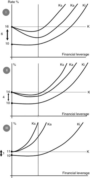
Figure 7.2 Return on Equity in Three Firms Facing Different Rate of Return on Total Investment
We can conclude that since firms have no or little control over the cost of debt, they can always widen the differential by obtaining a higher rate of return on their investment through better diversification, smarter management, and innovative production.
The Modigliani–Miller Approach
The basic premise of the Modigliani and Miller thesis was that there is no optimal capital structure, and moreover, that capital structure would not be able to affect the firm's value. The reason is summarized by the compensatory effect of the market value of the firm's stock that would decrease any time the firm incurs more debt and gets into a higher level of risk. It is because the firm's market value is actually the sum of the market value of debt and market value of stock.
Modigliani and Miller separate between the firm's value and its cost of capital, on one hand, and the form of capital structure on the other. They attribute the firm value to its ability to obtain the highest expected return on investment, utilizing the best capitalization rate, given that:
- The capitalization is for the firm's pure equity stream for a certain class with a proper consideration of the potential financial risk.
- The capitalization rate would not be related to the type of securities that would be utilized for investment.
- Finally, their argument gave a lot of weight to the personal arbitrage and its ability to change the dynamics of the financial leverage.
Other Approaches to Capital Structure
Both the traditional and Modigliani–Miller approaches to capital structure have been criticized for not being able to help the small business particularly. The criticism is specifically based on the notion that it would be difficult for a small business to calculate its cost of capital. Other alternative approaches such as the EBIT–EPS have been introduced to be a better fit for the small business.
The EBIT–EPS Approach
This approach utilizes the firm's EBIT as well as its earnings per share (EPS). Table 7.3 presents data for a firm considering three plans for capital structure. Plan I uses 25% debt and 75% equity splitting the entire capital of $400,000 between $100,000 debt capital and $300,000 equity capital. Plan II uses a 50:50 split between debt and equity, and Plan III uses a 75% debt and 25% equity making debt capital equal to $300,000 and equity capital equal to $100,000. It is assumed that the interest on debt would increase as the amount borrowed increases so that 10%, 12%, and 15% interest rate go with the three plans, respectively. Taxes are assumed to be 15%, and stock price is $10 per share. Number of outstanding shares are concluded as 30,000, 20,000, 10,000 shares for the three plans, respectively.
Table 7.3 Three Plans for Capital Structure
| 1 | 2 | 3 | 4 | 5 | 6 | 7 | 8 | |
| Plans | Capital Structure D:E | Debt Capital | Equity Capital | Total Capital 2 + 3 | Interest Rate on Debt (%) | Total Interest on Debt 2 × 5 | Stock Price ($) | No. of Shares 3 ÷ 7 |
| I | 25:75 | 100,000 | 300,000 | 400,000 | 10 | 10,000 | 10 | 30,000 |
| II | 50:50 | 200,000 | 200,000 | 400,000 | 12 | 24,000 | 10 | 20,000 |
| III | 75:25 | 300,000 | 100,000 | 400,000 | 15 | 45,000 | 10 | 10,000 |
Table 7.4 picks two arbitrary amounts of EBIT, $50,000 and $100,000 and calculates the EPS for each plan of capital structure using the information in the previous table. Once we get two coordinates from each plan, we can draw the three plans as straight lines which would be used to compare alternative capital structures from which the firms would know the best. We can see which and where any plan line would be superior or inferior to each other. Figure 7.3 shows that up to $50,000 EBIT, Plan I line is above Plan II line, meaning that at such a phase of the firm's operation, it would be more productive to use a capital structure of  debt and
  equity. For EBITs between $50,000 and $66,000, the firm should favor the 50:50 debt/equity capital structure since Plan II is above the other two plans. For EBIT above $66,000, it seems like more debt such as
  of the total capital would be better than any other capital structure. It would yield an EPS of 4.68 and higher.
Table 7.4 The Effect of Selected EBIT on EPS Across the Three Plans of Capital Structure
| Plans | EBIT | Interest | Earnings after Interest | Taxes 15% | Earnings after Interest and Taxes | No. of Shares | EPS |
| I | 50,000 | 10,000 | 40,000 | 6000 | 34,000 | 1.1 | |
| 100,000 | 10,000 | 90,000 | 13,500 | 76,500 | 30,000 | 2.55 | |
| II | 50,000 | 24,000 | 26,000 | 3900 | 22,100 | 1.1 | |
| 100,000 | 24,000 | 76,000 | 11,400 | 64,600 | 20,000 | 3.23 | |
| III | 50,000 | 45,000 | 5,000 | 750 | 4250 | 0.425 | |
| 100,000 | 45,000 | 55,000 | 8250 | 46,750 | 10,000 | 4.68 |
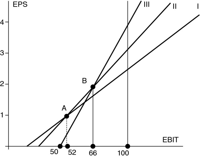
Figure 7.3 Three Plans for Capital Structure
Points A and B are called the indifference points: the points of intersection of two or more capital structure plan lines that would occur at a certain level of EDIT, the intersecting plans would produce the same EPS. This is why a manager would be indifferent as what capital structure plan is used since they result in the same level of EPS. The following formula can be used to find the indifference point (ip):

where
- I1: Total interest in Plan I
- I2: Total interest in Plan II
- S1: Number of shares in Plan I
- S2: Number of shares in Plan II
We can use data from Plan I and Plan II to get point A, and data from Plan II and Plan III to get point B.

Since indifference point B is between Plan line II and Plan line III, the formula should be

It should be mentioned here that the EDIT–EPS approach does not guarantee any optional capital structure for the firm but it would certainly offer a general guideline for the managers by which they gauge the proper amount of debt that would not hurt the firm's major financial objectives.
EBIT–EPS and Risk Indication
Although the risk can be indicated by calculating the standard deviation from the expected EBIT, risk also can be viewed by both the indifference point and the slope of the plan line. There is a positive relationship between the indifference point location and risk level on one hand and between the slope of the capital structure plan line and risk on the other hand. The higher the point and steeper the line, the higher the expected risk level.
Also, the TIE ratio can be calculated to indicate the risk level where the relationship between this ratio and risk is negative. The lower the TIE ratio, the higher the risk. We can calculate this ratio for the EBIT level of 100,000 using the total interest paid on debt for the three capital structure plans.

Since the lowest ratio is with Plan III, this capital structure is the most risky which emphasizes the conclusion that the risk level would increase as the firm uses more financial leverage.
Last, but not least, it should be known that this approach has been criticized for many reasons, the most important of which is that the depiction of the plan lines assumes that both interest rate on debt and tax rate on earnings remain constant throughout the changes of earnings and debt levels, which can be false in reality.
7.3 Leverage
Leverage generally refers to a more than proportional change in one variable in response to a certain change in another related variable. In high school physics we learned the concept of leverage in the use of a lever to lift a mass of high weight using a minimized amount of force. In social and political context, we learned that having more leverage meant having the ability to accomplish a lot with the power of a small action or word. In an economic sense and in the business world, leverage would mean the effects of small changes in the fixed-cost assets or funds on the firm's earnings. There are three kinds of leverage: operating leverage, financial leverage, and combined or total leverage.
Operating Leverage
Operating leverage refers to the responsiveness of the change in profits due to the change in sales. Specifically, it is the potential use of fixed operating costs to magnify the effects of changes in sales on operating income and EBIT—the fixed operating cost being those items at the top of the balance sheet such as leases, executive salaries, property taxes, and the like.
Degree of operating leverage (DOL) measures the responsiveness of profit as a percentage change in operating income (OY) relative to the percentage change in sales (S).


Example Table 7.5 shows that the operating income of a small business increased from $884 to $1680 as it expanded the sales of its product from $4200 to $5880, what would be the degree of its operating leverage?
| S | OY | ||
| S1 | 4200 | 884 | OY1 |
| S2 | 5800 | 1680 | OY2 |
This means that for every 1% change in sales, there would be a 2.25% change in operating income (profit or EBIT). In other words, as sales increased by 40%, profits rose by 90% as is shown in the denominator and numerator of the DOL, respectively. It is also shown in Figure 7.4. The move from Q1 to Q2 on the units of sale (or R1 to R2 on the dollars of revenue) would result in the move from Prof1 to Prof2. This effect would hold the same in the other direction, meaning that a reduction in sales (units of product or dollars of revenue) by 40% would result in a drop in the profit by 90%. We can calculate a move in sales in the opposite direction from Q1 to Q0 or in revenue from R1 to R0 which is about 40% less (420 to 252 units or $4200 to $2520) and see the profit drop 90% from Pr1 = 884 to Pr0 = 88.4.


Figure 7.4 The Effect of Change in Sales on Profit
So, the DOL can actually be considered a multiplier of the effect that a change in sales would have on profit. In other words, DOL is a concept of elasticity. It is the elasticity of profit with respect to sales. In such a sense, we can express it as the partial change in profit (π) relative to the partial change in output (Q).

The degree of leverage can be obtained at any level of output. If fixed cost is constant, the change in profit (∂π) would be

Also profit π is

Substituting (1) and (2) in the DOL equation above,

Cancelling out ∂Q, we get

which is the DOL at any level of output.
Example Find and interpret the degree of operating average DOL for a firm which has the following data:
- FC = $2500
- Variable cost per unit = $5
- Unit price = $10
- Units of product sold = 1000

The DOL is 2 means that for every 1% change in sales, operating income would change by 2%.
Operating Leverage, Fixed Cost, and Business Risk
A major observation can be made on the above DOL formula. This observation is related to the fixed operating cost and its effect on DOL. Mathematically, since the term Q(p − v) is present in both the numerator and the denominator, the role of fixed cost (FC) becomes crucial. Any increase in FC would make the denominator less and the DOL higher, and any decrease in FC would make the denominator more and DOL lower. We can then conclude that the higher the firm's fixed operating cost, relative to its variable cost, the greater the degree of freedom and ultimately the higher the profit. Let us try this by observing the change in DOL if the fixed cost in the last example increases from 2500 to 4000.
A 5 degree of leverage means that the profit would increase by 5% instead of 2% when the sales increased by 1%. Table 7.6 and Figure 7.5 shows how the DOL and the profit (Pr) would change as the fixed cost increases notably across three firms selling the same product for the same price. However, as we have seen before, operating leverage works in the opposite direction too. This means that if we take the figures of the previous example, a decrease in sales by 1% would be more damaging by lowering profits by 5%. So, the increase in the fixed cost would really make the situation more sensitive in both ways, which can translate into presenting a source of business risk. Such a potential risk can come from two sides.
- In the case of seeking more profits through the increase in the fixed cost, the firm would take the risk of not being able to cover all of the high cost and additional risk of not being able to maintain the increase in sales.
- In the case of a slight drop in the sales, the firm would take a risk of facing its profit dropping significantly. It may drop to the point to threaten any reasonable recovery.
Table 7.6 Fixed Cost Increase and DOL in Three Firms
| Q | R | Cost = FC + VC | Pr | Change in Pr (ΔPr) |  |
||
| Firm 1 | Break-even | 1000 | 3000 | 3000 | 0 | 0 | FC = $1000 vc= $2.00 |
| 1500 | 3500 | 4000 | 500 | 500 | P = $3.00 | ||
| 2000 | 6000 | 5000 | 1000 | 500 | |||
| 2500 | 7500 | 6000 | 1500 | 500 | |||
| 3000 | 9000 | 7000 | 2000 | 500 |  |
||
| → 3500 | 10,500 | 8000 | 2500 | 500 | |||
| 4000 | 12,000 | 9000 | 3000 | 500 | DOL = 1.4 | ||
| 1000 | 3000 | 4000 | −1000 | FC = $2250 vc = $1.75 | |||
| Firm 2 | Break-even | 1800 | 5400 | 5400 | 0 | −1000 | P = $3.00 |
| 2500 | 7500 | 6625 | 875 | 625 | |||
| 3000 | 9000 | 7500 | 1500 | 625 | |||
| → 3500 | 10,500 | 8375 | 2125 | 625 |  |
||
| 4000 | 12,000 | 9250 | 2750 | 625 | |||
| 4500 | 13,500 | 10,125 | 3375 | 625 | DOL = 2.06 | ||
| 1000 | 3000 | 5000 | −200 | FC = $3750 vc = $1.25 | |||
| Firm 3 | Break-even | 2143 | 6429 | 6429 | 0 | −2000 | P = $3.00 |
| 2500 | 7500 | 6875 | 625 | 625 | |||
| 3000 | 9000 | 7500 | 1500 | 875 | |||
| → 3500 | 10,500 | 8125 | 2375 | 875 |  |
||
| 4000 | 12,000 | 8750 | 3250 | 875 | |||
| 4500 | 13,500 | 9375 | 4125 | 875 | DOL = 2.58 |

Figure 7.5 Fixed Cost Increase and DOL in Three Firms
So, the ever-increasing temptations to benefit from the new technology, modernize production, and replace labor-intensive by capital-intensive technology would most likely increase efficiency but require incurring a lot more fixed cost which, if done, has to be with much more caution and consideration by financial managers who have to carefully and rationally weigh the benefits of increasing the profits with all of the risks associated with them.
Financial Leverage
The financial leverage refers to the responsiveness of the change in the firm's EPS to the change in its operating income (profit) or EBIT. Similar to the operating leverage, the financial leverage expresses the potential use of fixed financial charges to magnify the effects of changes in operating income (OY) on EPS—the fixed financial charges here being specifically interests on debt and dividends for preferred stocks. These are the liabilities at the lower part of the balance sheet. In other words, financial leverage is mainly about financing businesses, totally or partially, by debt and it is no surprise that the financial leverage approach is sometimes popularly called “OPM” or other people's money and also called “trading on equity” or “debt financing.” Using debt in business investment typically comes from rational reasons such as:
- The returns on debt investment are higher than the returns on equity investment.
- Debt capital is most likely to be readily available.
- Using debt capital usually does not affect the voting situation in the firm.
In a nut shell, if a firm has a high fixed cost of financing, it would be considered heavy on financial leverage, and most likely enjoy high returns on investment but would, in turn, face potential financial risks.
Just like the operating leverage, financial leverage has its own degree, and it is called “degree of financial leverage” or DFL. It measures the sort of responsiveness of the change in EPS relative to the changes in operating income (OY).


Note that EPS refers to the net earnings that would be distributed to common stockholders.
and if there are any preferred stocks, their dividends have to be deducted from net income before obtaining the EPS.
| Item | Year 1 | Year 2 |
| Gross income | 30,250 | 32,900 |
| Operating expenses | 10,100 | 10,940 |
| Interests | 766 | 870 |
| Income taxes | 3400 | 3490 |
| No. of shares | 30,000 | 30,000 |
Example Calculate the DFL in the Sureluck Company whose data for two consecutive years is showing in Table 7.7 above.
First, we need to calculate OY and EPS.

For EPS, we need to calculate net income by deducting interests and taxes from the operating income.

As shown in Table 7.8, we can calculate EPS as:
| OY | EPS | ||
| OY1 | 20,150 | 0.53 | EPS1 |
| OY2 | 21,960 | 0.59 | EPS2 |
The DFL of 1.26 means that for every 1% change in Sureluck's operating income, there would be a 1.42 change in its EPS. This would be true for the increase or decrease in the EPS that would respectively follow the increase or decrease in the operating income.
Example Let us assume that the Sureluck Company in the last example distributed about 43% of its net income as dividends for preferred stocks. How would that affect the DFL?
The change would be in the calculation of the EPS. The preferred stock dividends have to be deducted from net income before dividing that net income among the common shareholders.


There is another formula for DFL at a base level of operating income. It is more direct when preferred stock dividends are paid. With this formula we would not have to calculate EPS.
Where OY is operating income, I is interest, Dps is dividends for preferred stocks, and T is income tax rate.
If we calculate the DFL of the previous example, we need to know the income tax rate. But we can, for this purpose, assume it based on the relation of taxes to income. So, let us just assume that the tax rate in this example was 16.8% for year 1, and 15.9% for year 2. We can now calculate the DFL individually for each year based on their operating income.

Example In this example we will follow the impact of financial leverage on EPS throughout three possible alternatives of financial plans. Let us assume that a firm needs $100,000 to expand its business, and let us assume that the firm board has the following alternative plans to finance this expanding project.
- Plan I: 100% equity financing. The entire $100,000 would be obtained by selling 1000 shares at $100 each.
- Plan II: 2/3 equity financing and 1/3 debt financing. That is 66% of the $100,000 ($66,000) would be obtained internally, and 34% ($34,000) would be obtained by borrowing at 9.5% interest.
- Plan III: 1/3 equity financing and 2/3 debt financing. That is 34% ($34,000) would be obtained internally and 66% ($66,000) would be a business loan at 9.5% interest.
In Table 7.9, we see the data for these three financial plans. We are assuming that operating income is 20% of the capital employed, and taxes are 40% of the earnings after interest. We are allowing the operating income to increase and decrease by 25% in each of the plans. Number of shares is assumed to be 5000.
Table 7.9 Three Plans to Finance an Expansion Budget of $100,000
| Financing Plans | Total Capital | Equity Part (EQ) | Debt Part (D) | Operating Income (OY) | Interest 9.5% (I) | OY − I | Taxes 40% (T) | Net Income (NY) (OY-I-T) | Return on Equity (NY/EQ) (%) | EPS (NY/#S) | DFL |
| Plan I | 100,000 | 100,000 | 0 | 20,000 | 0 | 20,000 | 8000 | 12,000 | 12 | 2.40 | |
| OY 25% ↑ | 100,000 | 100,000 | 0 | 25,000 | 0 | 25,000 | 10,000 | 15,000 | 15 | 3 | 1.25 |
| OY 25% ↓ | 100,000 | 100,000 | 0 | 15,000 | 0 | 15,000 | 6000 | 9000 | 9 | 1.8 | 1 |
| Plan II | 100,000 | 66,000 | 34,000 | 20,000 | 3230 | 16,770 | 6708 | 10,062 | 15.2 | 2.01 | |
| OY 25% ↑ | 100,000 | 66,000 | 34,000 | 25,000 | 3230 | 21,770 | 8708 | 13,062 | 19.8 | 2.61 | 1.49 |
| OY 25% ↓ | 100,000 | 66,000 | 34,000 | 15,000 | 3230 | 11,770 | 4708 | 7062 | 10.7 | 1.41 | 1.19 |
| Plan III | 100,000 | 34,000 | 66,000 | 20,000 | 6270 | 13,730 | 5492 | 8238 | 24.2 | 1.65 | |
| OY 25% ↑ | 100,000 | 34,000 | 66,000 | 25,000 | 6270 | 18,730 | 7492 | 11,238 | 33 | 2.25 | 1.82 |
| OY 25% ↓ | 100,000 | 34,000 | 66,000 | 15,000 | 6270 | 8730 | 3492 | 5238 | 15.4 | 1.05 | 1.45 |
The data shows that as the firm uses debt to finance the expansion project, returns on equity rose in increasing rates from 15.2% in Plan II to 24.2% in Plan III. That is by 60%. Also, as operating income increased by 25%, return on equity increased by 30% (from 15.2% to 19.8%) in Plan II and by 36% (from 24.2% to 33%) in Plan III. It is also evident that an increase in leverage caused the EPS to increase. This is to say that the increase in EPS relative to 1% increase in operating income is shown by the DFL, increasing throughout the plans from 1.25 to 1.49 to 1.82. Conversely, the decrease in leverage caused the EPS to decline. Also, the effects of both the income and decrease in income on EPS were more dramatic as we move from Plan II to Plan III that uses a higher debt.
Total or Combined Leverage
We have seen that changes in sales revenues have caused greater changes in the firm's operating income which, in turn, has been reflected in changes in the EPS. It is logical to conclude that using both operating leverage and financial leverage would highly affect the firm's EPS. Therefore, the combined effect of both types of leverage is what we call the “total leverage.” It is defined as the potential use of both operating and financial fixed costs to magnify the effect of changes in sales on the firm's EPS. Figure 7.6 shows the connection between sales and EPS through the changes in operating income or EBIT utilizing the two kinds of leverage, operating and financial.

We can see that an ultimate link between the changes in sale revenue and the variations in the EPS can be visualized as the line of combined or total leverage.
The degree of combined leverage (DCL) can be obtained as a product of the DOL and the DFL.

Canceling out %ΔOY, we get
Example In the last 2 years, a small firm managed to increase its sales revenue from $88,000 to $96,000. Its EPS have also been increasing from 1.05 to 1.56. What would be the DCL?


This means that for every 1% change in the firm's sales, EPS have changed by 5.34%, we can also use the following formula to obtain the degree of combined or total leverage:

where Q is a given size of the product, P is the price of a unit of production, v is the variable cost per unit of production, FC is the fixed cost, I is the interest, Dps is the dividends for preferred stocks, and T is the tax rate.
Example A firm faces $6000 fixed cost and $1.50 variable cost per unit. It pays $8210 as interest on its debt, and pays income taxes at the rate of 36% and $10,000 in dividends for preferred stock. What would be the degree of its combined leverage if it sells 15,000 units at $6.50 each?

7.4 Summary
This chapter on capital structure and leverage started with defining capital structure and explaining how the term practically meant the makeup of capital in a firm to finance its operation. It revealed that the capital makeup often meant the percentages of debt capital and equity capital. The chapter then explained both types of capital starting with debt capital and its three categories that are classified based on the extension of time for the debt payment. The three subcategories were the short-term, the intermediate, and the long-term debt. Next was equity capital that went over the owner's own investment and the contributions by other investors including the venture capitalists and angel investors. A comparison between debt and equity capital was made and a detailed numerical example was given to illustrate that a firm might prefer to finance its operation by debt versus equity capital.
On the optimal capital structure, several theoretical approaches were explained including the traditional approach, the Modigliani–Miller approach, and the EBIT–EPS approach. Math and graphs were used to illustrate the main points, as well as assess the risk. Leverage was the last section in this chapter. Both operational and financial leverage, as well as the combined leverage were articulated with math, graphs, and numerical examples. Those examples focused on how to measure the leverage through three different criteria called the degrees. These degrees were respectively the DOL, DFL, and DCL.
Key Concepts
- Capital structure
- Debt capital Equity capital
- Short-term debt
- Intermediate-term debt Long-term debt
- Short-term bank loan
- Trade credit Venture capitalist
- Angel investor
- The traditional approach Modigliani–Miller approach
- EBIT–EPS approach
- Leverage Operational leverage
- Financial leverage
- Combined leverage Degree of operational leverage (DOL)
- Degree of financial leverage (DFL)
- Degree of combined leverage (DCL)
- Other people's money (OPM)
- Trading on equity Debt financing
Discussion Questions
-
What is meant by capital structure, and why is it important?
-
What is debt capital and equity capital, and how would a firm decide to depend on any of them?
-
Which capital is often preferred by the owner-manager and why?
-
What are the criteria to classify types of debt capital?
-
Is there anything such as an optimal capital structure? And what did the different experts say about that?
-
Briefly explain the traditional approach on optimality of capital structure.
-
How is Modigliani–Miller approach different from the traditional approach?
-
What is leverage? And why would a firm need it?
-
Briefly explain the difference between operational leverage and financial leverage, and the ways they are measured.
-
What is combined leverage? And what would it measure?