CHAPTER 8
PROFIT AND THE COST–VOLUME ANALYSIS
8.1 Profit Concept Between Economics and Accounting
There is no doubt that “profit” is the most common and widely used term in the business world. However, the commonality and popularity of the term does not necessarily make it a clear concept with an unequivocal connotation. When the classical economics specified the four major factors of production as land, labor, capital, and entrepreneurial management, it also specified the payments these factors get for their individual contribution in the production process. These payments are respectively: rent, wages, interest, and profit. From here we can conclude that profit is the monetary return to those who initiate and manage the entrepreneurial function of production. If the first three payments (rent, wages, and interests) are made out of the product's sale revenue, the residual, if any, would constitute the fourth payment to the entrepreneur or owner as profit. It is in this sense we get the equality between profit and the net revenue since what we call profit is in fact the surplus over and above the costs of production. These costs may also include taxes, financing cost, and the like. Technically, profit would equal the difference between the total cost of production (TC) and the total revenue brought by the sale of products (TR).

It is worthwhile to note here that while the term total revenue is a clear and well-defined concept, the total cost is less clear. Total revenue is the dollar value of the product sold, which is obtained by multiplying the quantity of the units of products sold by the market price per unit. Total cost could include only the explicit cost or the outlay such as the expenditures on the factor of production mentioned earlier and other direct payments such as taxes and interests on loans. If the total cost includes only the explicit cost (EC), the calculated profit would be considered as business or accountant's profit (πa).

Total cost could also include the implicit cost in addition to the explicit. The implicit cost (IC) is represented by the opportunity cost of the used resources. If that is the case, then the calculated profit would be called the economic profit (πe).

Economists tend to consider the foregone value of resources that would have been earned had they been used in any alternative purpose.
Since the accountant's profit is a straightforward and direct concept in its measurement, it is used in the business books. The economic profit, on the other hand, would be more suitable for the purpose of decision-making and risk and return assessments.
Profit can very well measure the efficiency of a business. As firms pursue their self-interest, the mechanism of profit maximization would work wonders on the allocation of resources. By such a mechanism, resources would be automatically moved toward the production of goods and services that are most valued and demanded by society. Over time, firms which are making fewer profits would leave their projects and seek to employ their resources in more profitable endeavor and may enter more lucrative markets. Eventually, collective market efficiency would be established and aggregate welfare would be achieved. Profit and profitable projects and sectors would ultimately indicate business efficiency while losses would signal the lack of efficiency.
8.2 Profit Margin and Markup
Based on another distinction among the cost concepts, profit would also be classified as gross and net. Gross profit is the difference between total revenue and cost of production only, while net profit is the difference between total revenue and all costs including production costs and all other costs such as taxes and interests paid and others. If either gross profit (GP) or net profit (NP) is divided by revenue (R), we would get gross profit margin (GPM) or net profit margin (NPM).

NPM is often used internally to generally indicate the extent of safety and control over costs, prices, and marketing strategies. It is not to be confused with the markup, which is often the case. Markup, as an absolute amount (MA), is the difference between the cost of a product (C) and its selling price (Ps). In retail business it is the difference between the retail price (the consumer's cost) and wholesale price (the retailer's cost). Often it is a desired amount or percentage that is set up by the retailer in advance.
Example Suppose that handmade dolls are made by a home business. Each doll costs $12.00 and it is sold in the market for $20.00. The markup amount would be $8.00.

Markup also can be expressed as a percentage either out of the selling price (8.00/20.00 = 40%) or out of the cost (8.00/12.00 = 66%). In retail business the markup percentage is often calculated out of the wholesale price, which is the retailer's cost.

For an entrepreneur who would like to decide a certain markup percentage over the cost of product, and would want to know how much the product should be sold to achieve that desired markup, we can solve the last equation for the selling price (Ps).
Example An entrepreneur calculated the cost of his product as $625 per unit. He would want to sell it so that he can get 55% markup. How much should he price his product?

Example Suppose that a retail store offered the entrepreneur above to sell his product in the store for $850. How much markup the entrepreneur would get, and what markup percentage would that be?
It can also be obtained by
Markup can also be expressed as a percentage of selling price (Ms%).

We can go back between Mc% and Ms% by following the formulas below.


Example A small company sells its product for $25 when its cost is $10. What would be the percent markup based on the product cost, and the percent markup based on the selling price, and how would we go back and forth between the two percentages?
As for how the profit margin is connected to markup, we should recall that profit margin (PM) is obtained by dividing profit by revenue, where profit is the difference between revenue and cost.
But that is in an aggregate sense, which could also be reduced to a per unit sense where profit per unit would be the difference between selling price (Ps) and the product cost per unit (C), and the revenue of one unit would be its selling price. Therefore, the profit margin per unit (PMpu) would be

But since the top is nothing but the markup amount (MA), the profit margin per unit would become the ratio of the markup amount to the selling price.

We can also go further this way.

Example Calculate the profit margin for the entrepreneur of the last example and verify your answer.

The profit margin would be
8.3 Profit and Cash Flow
Cash flow is the money streaming into and out of the business over time. It is an indication of the firm's liquidity and its capacity to run monetary transactions and pay for its contractual obligations and bills on time. As Figure 8.1 shows, there are two continuous streams of cash: the cash inflow in the upper panel represents all the money that the firm receives, which includes
- – Capital funds: the immediate investment and the allocated investment along the way.
- – Investment earnings, which include what the firm is currently earning on its external investment and what is expected to be earned later on.
- – Asset sales, which is what the firm obtains for selling some of its assets either by cash or credit.
- – Product sales that include the firm's revenues from selling its products and services for both cash and credit.
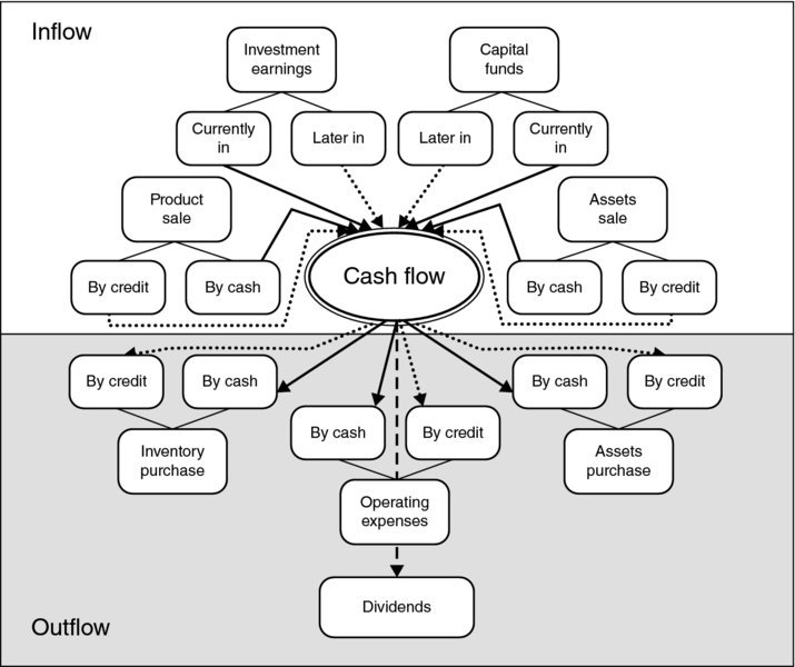
Figure 8.1 Cash Flow Diagram
The lower panel of the figure represents the cash outflow or what the firm spends, which includes
- – all the operating expenses on all products and services, and obligations necessary to produce, market, and sell the firm's product such as buying material, hiring labor; paying for land, buildings, and machines; promotion and advertising, servicing loans, buying insurance, paying for taxes and all other needed purchases, whether it is paid by cash or credit;
- – purchases of inventoried material;
- – purchases of assets;
- – and ultimately what the firm pays for its shareholders as dividends.
The state of cash flow is never static. It is changing continuously as both in and out streams are flowing day by day. This is the fact that gives significance to the net cash flow, which is the difference between cash inflow and cash outflow at any point in time. It is the net cash flow that is being confused with the profit since profit is the difference between revenue and cost of operation, and is sometimes called net income for the entrepreneur. Net cash flow and net income (profit) are simply not the same! There are three reasons to explain why they are not the same.
- A major reason is the timing element that plays a crucial role in setting the status of cash flow at any point in time. Figure 8.1 shows two kinds of arrows, the solid for the immediate transaction, in and out, and the dotted for the delayed transactions, in and out. For example, when a firm's records show $5000 of product sale on a certain day, it may mean that only $1500 is actually in for the cash sale while the rest of $3500 is not in yet and it might take another month or two to be received for being a credit sale. It could also be less than $3500 when it is depending on what portion of it is collectible and what is not. Similar differences may also happen with the expenses. A firm may decide to pave the driveway and parking lot for $20,000 but it would disperse only $10,000 initially, leaving the balance of $10,000 to be dispersed in two installments of $5000 over the next 2 months. Taking the timings of all inflows and outflows into consideration, we begin to see how fluid the state of cash flow is.
- Another reason to separate between profit and net cash flow is the fact that some major components of the inflows, such as the capital fund and external investment earnings, cannot be considered revenue as long as they are not generated due to the sales of the firm's products or services.
- Yet another compelling factor to distinguish between profit and net cash flow is the fact that a positive net cash flow is essential for the firm to operate because it is the life line that maintains the firm's ability to pay its bills. A firm, however, can very well operate and survive for a certain time when it has no profit or even negative profit (loss).
8.4 Profitability and Earning Power
Profitability (PT) is the ability of the employed assets to generate profit. It is also defined as the return on assets (ROA) or return on investment (ROI). Profitability can, therefore, measure the efficiency of a business. Technically, profitability can be obtained by dividing net profit (NP) by the total assets (TA) or total investment.

Example Suppose that a firm's total assets for making auto parts is $400,000 and for auto repair is $90,000. Its net profit in the manufacturing section is $130,000 and in the repair shop is $65,000. Which business section is more profitable and more efficient?
In the manufacturing department, profitability would be
and in the repair shops, profitability would be
which means that running the auto repair shop would be more efficient and profitable than continuing with part manufacturing, which racked up more than four times the amount of investment in assets than it did in the repair shop.
The other face of business efficiency is represented by what is called “earning power,” which is defined as the firm's ability to generate profits through maximizing sales revenue out of its assets utilization. Technically, the earning power (EP) is the mathematical product of two elements: The first is the NPM and the second is the total asset turnover (TAT).

We know that NPM can be obtained by dividing net profit (NP) by sales revenue (R). TAT refers to the firm's capacity to utilize its assets and generate the highest revenue out of them. It is obtained by dividing sales revenue (R) by total assets (TA). If we substitute for these two elements in the earning power equation, we get
Cancelling out (R) would give us

and that is how we obtained profitability (PT).
This is why profitability and earning power are two different terms referring exactly to the same thing, that is, how successful the business is in using its resources and assets, getting the right sales and right revenue to maximize its profits.
Figure 8.2 depicts the status of earning power in a business. Businesses on any higher point of the curve, such as A, would have a larger earning power and higher efficiency by enjoying a high level of profit margin (npm2) and low level of asset turnover (tat1). Alternatively, businesses on any lower point of the curve such as (B) would get a lower level of net profit margin (npm1) and high level of asset turnover (tat2). Businesses that are anywhere between A and B would have different combinations of NPM and asset turnover, and their efficiency or profitability would be less than that of A and more than that of B.

Figure 8.2 Status of Earning Power in a Business
8.5 When Would a Firm Start Collecting Profits?
Although the central objective for any for-profit business is to make profit, it is essential for those businesses to understand and recognize the timing at which profits can be collected. For a starter, common sense dictates that all costs of production must be covered first. The firm has to price its product and sell it so that it can collect the volume of revenue that would first and foremost cover the cost of producing and marketing the product. To get to this point is to achieve what is called the break-even point. That is when the firm is able to even out its costs with its revenues.

This is the point that marks the end of incurring losses and the start of collecting profits, given that the firm would continue selling its product and collecting more revenue that would exceed covering the total cost. Any access revenue over covering the cost would be considered profits. Finding the point that equates the costs with revenues is called the break-even analysis or the cost–volume–profit analysis. The point can be expressed in production size by units of product, or in the monetary value by number of dollars, or by time units.
Cost–Volume–Profit Analysis
The cost–volume–profit can be defined as the process determining the level of output that must be produced and sold before any profit can be earned. It can also be the determination of the amount of revenue that can be collected before earning any profit. The reliance on finding the revenue instead of the production size can be more practical and convenient if the firm produces or sells multiproducts. For example, General Motors can easily determine how many Chevy Malibu, for example, should be sold before that plan starts to earn profits, but this method cannot be easily used for Walmart, because Walmart stores sell tens of thousands of products. It is, therefore, more appropriate to determine how much sales revenue should be collected before a certain Walmart store starts to earn profits.
The major objective of the cost–volume–profit analysis is to identify a specific output level which would first and foremost be able to cover the fixed cost of production. It is considered an important tool for business performance and profit planning that utilizes the restructuring of the fundamental relationship between cost and revenue. This analytical tool offers the manager or business planner a plausible approximation of the point when profits begin to be collected according to the realization of the state during which the total cost of production has been recovered by revenues from the production sales.
Technically, the cost–volume–profit analysis is to find the point that refers to both the break-even quantity (BEQ) of product and the break-even revenue (BER) of sales. This break-even point is where the profit would be equal to zero and the total cost would equal to total revenue. Geometrically, it is the point of intersection between TC and TR curves. Once we locate this point, we would know that all production before that point incurs some loss and any product produced and sold after that point would yield some profits. Before we identify the mathematical expressions in this analysis, we should be able to know the operational definitions of the variables involved. The variables are what constitute both the cost and the revenue. Of special importance to clarify is that the cost components for it are imperative to distinguish between what is fixed and what is variable cost, before solving any break-even problem.
Total Cost
Total cost (TC) of production includes both fixed cost (FC) and variable cost (VC).

Fixed Cost (FC): Fixed costs are the costs that are not associated with the size of production or sales of products. They are a function of time, not sales or production, and therefore they are incurred whether or not the firm produces anything or sells any product. Typical examples of the fixed costs are rent, lease payments, insurance premiums, regular utilities, executive and clerical salaries, and debt services. All these are expenses that have to be paid regardless of how much the firm produces or sells. Geometrically, they are represented by a horizontal line.
Variable Cost (VC): Variable costs are any costs that are tied to size of production or sale. They fluctuate up and down positively with the volume of production or sales. Typical examples of the variable costs are production materials, production labor, and production utilities such as the cost of electricity and gas consumed by the productive machines and equipment, merchandise insurance, transportation, and storage. The more the firm produces, the more this kind of costs incurs. In this sense, VC would be a product of the size of production (Q) and the cost per unit of a particular product (v).

Total Revenue
Total revenue (TR) is the proceeds collected out of selling the goods and services produced by the firm. It is obtained by multiplying the quantity of the product sold (Q) by the market price per unit of the product (p).

Contribution Margin (CM): Contribution margin is the amount of profit earned on each unit sold above and beyond the BEQ, and similarly, it would be the amount of loss the firm would incur on each unit produced below the break-even point. Technically, it is equal to the unit price of the product discounted for the unit variable cost. Mathematically, CM would be

and that is, in fact, the denominator of the BEQ formula that we will see next.
8.6 Break-Even Quantity and Break-Even Revenue
If the total cost (C) includes both FC and VC, then

Since VC changes with the size of production, let us consider v as the variable cost per unit of production. If production is Q, then

and

Also, revenue (R) will depend on how many units of product are sold. If we consider p as the price per unit of product, then

Profit (Pr), sometimes called operating profit or earnings before interests and taxes (EBIT) is the difference between total revenue and total cost, then

and since profit is zero at the break-even point


This Q is the quantity of products at the break-even point, and it is called the BEQ.

where again, FC is the fixed operating cost, p is the price per unit of product, and v is the variable operating cost per unit of product.
Similarly, we can find the revenue at the break-even point.
Let us start with Equation 2.

We substitute for the Q value that is obtained from Equation 1.


At the break-even point Pr = 0


This is the revenue at the break-even point, and it is called the break-even revenue (BER).

By knowing the BEQ or BER, a firm can
- determine and control its operations in order to sustain the proper level of output to cover all operating costs;
- assess and control its ability and timing to earn profits at different levels of production and volumes of sale.
Example If a business incurs $5620 fixed cost and $1.20 variable cost per unit, and it sells its product for $8.75, how many units of the product have to be produced and how much revenue has to be collected before this business starts earning a profit?
Solution


and


BER can also be obtained by calculating the monetary value of BEQ.


Example Table 8.1 shows the records for a company that designs custom scrapbooks and sells its service for $40 per book. Calculate the break-even quantity and the break-even revenue.
Solution
- – The first task is to separate FC and VC on the basis of our understanding of the concepts. In this case, fixed and variable costs should be identified.
- – Fixed costs are rent, property taxes, insurance administrative salaries, and employee benefits.
- – Variable costs are wages, paper, cardboard, glue, tape and thread, leather, ink and paint, and shipping and handling.
- – The second task is to unify the terms of the cost items. The standard is to convert every fixed cost item into annual, while variable cost items remain per unit.
Fixed costs, then would be

And variable costs would be


Also,


| Item | Frequency | Cost ($) |
| Rent | Monthly | 3360 |
| Property taxes | Semiannually | 1998 |
| Insurance | Quarterly | 1334 |
| Administrative salaries | Monthly | 7896 |
| Employees benefits | Annually | 6374 |
| Wages | Per book | 3.60 |
| Paper | Per book | 2.58 |
| Cardboard | Per book | 1.62 |
| Glue, tape, thread | Per book | 0.66 |
| Leather | Per book | 2.34 |
| Ink and paint | Per book | 1.14 |
| Shipping and handling service | Per Book | 2.40 |
8.7 Break-Even Graphics
Graphically, the break-even point (A) is the intersection point between total revenue curve, OR and total cost curve, FT. As is shown in Figure 8.3, total cost curve starts from point F where the fixed cost is represented by the horizontal FF. Total cost curve increases as the production size increases along the horizontal axis. This increase would basically reflect the increase in variable cost. The break-even point A corresponds to the BEQ, on the horizontal axis, and to the BER, on the vertical axis.

Figure 8.3 Break-even Point
Before BEQ, the firm would incur more cost than it can collect revenue. This is reflected by the segment FA of the total cost curve being higher than the segment OA of the total revenue. This would result in a loss estimated by the shaded area FOA that is increasingly narrowing until it would reach zero at point A. This is why the break-even point A is where the loss disappears and the profit starts to occur. After A and its corresponding point BEQ, the firm would start producing more and collecting more revenue that would rise above the cost making an excess that would be all profit. The area ART is an illustration of the increasing profit from point A and onward.
Since total revenue would increase if the price of unit increases for a given size of production, we can see on Figure 8.4 how the break-even point changes and how the dynamics of loss–profit would shift if the firm decides to have different pricing policy and charge higher or lower price per unit.
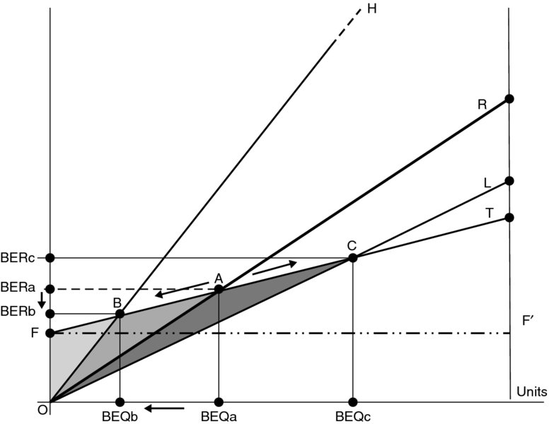
Figure 8.4 Break-even Point and Change in Price
Assuming that the total cost curve stays the same, raising the price per unit of product will result in a steeper total revenue curve than the previous OR such as OH. This would shift the break-even point left from A to B. This means that higher price means higher revenue for less production. BEQa would shift left to BEQb and so does BERa that would drop down to BERb. It would expedite the time to cut the losses and start collecting the profits. The loss area would shrink from FAO to FBO, and the profit area would expand from ART to BHT. Contrarily, if the price per unit is decreased, the total revenue curve would be flatter than the original curve OR. It would be something like OL, creating a new break-even point (C), which is to the right of the original point A. This new break-even point C would correspond to BEQc which requires larger size of production to compensate for the low price in reaching the BEQ. Although the BER would go up, C cannot occur but later, making the losses larger and the profits narrower. This may seem clear if we compare the loss area FCO to the profit area CLT.
As we know, any firm cannot randomly charge the price it wants at the time it chooses. The price is usually determined by the market conditions, which implies here that it would be more accurate if the total revenue curve is drawn based on the actual market demand on the product. Figure 8.5 shows the product sales curve OD as it bows down, reflecting the revenue fluctuations based on the demand law, where higher prices reduce the quantity demanded and yield lower revenue, and lower prices increase the quantity demand and bring higher revenue.

Figure 8.5 Break-even Point and Revenue Fluctuations
The introduction of the sales curve OD would allow us to see the profit areas more realistically. For example, if the product price is at a level to produce the total revenue curve OR and the break-even point is A, then the profit area would be to the right of A, between OR and FT, but under the curve OD. That area would be AEN. If the product price is lower to produce a flatter total revenue curve such as OL and the break-even point is C, then the profit area would be to the right of C, between OL and FT, and under the curve OD. This darkly shaded area would be the CMN. However, higher prices, such as those that would produce the total revenue curve OH and the break-even point B, would not result in any significant sales in the market and they would be beyond the curve OD.
8.8 Desired Profit and the Break-Even Point
Desired profit refers here to a certain amount that an entrepreneur would set up in advance to be targeted as an earned profit. It can technically be achieved by simply including it within the fixed cost. The formulas of both the BEQ and BER would then be adjusted by adding that desired profit to the top of the formulas along with the fixed cost.

and
where the subscript dp refers to the desired profit and DP is the desired level of profit.
Example If an entrepreneur wants to earn at least $80,000 on a project, the fixed cost of which is $42,000, the variable cost per product is $8.50 and the product sells in the market for $25.00. What would be the BEQ and BER?

Also,

Figure 8.6 shows how a predetermined profit can raise the break-even point and revenue beyond and above what they would have been when only the fixed cost was considered, as is normally the case.

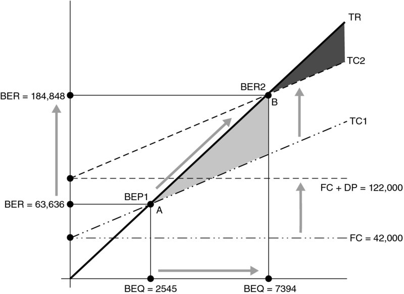
Figure 8.6 Break-even Point and a Pre-determined Profit
When only the fixed cost $42,000 was considered, the break-even point was at A, resulting in a BEQ of 2545 units of product and a BER of $63,636. But when the fixed cost was augmented by the predetermined profit of $80,000, the break-even condition was delayed, and the break-even point was shifted right to B. This has resulted in pushing the BEQ to 7394 units and raising the BER to $184,848. It is important to note that the shaded areas do not represent a comparison of the profit amounts as much as they show where each profit would start to be collected.
8.9 Non-Cash Charges and the Break-Even Point
Many firms may have to deal with non-cash elements of its operating cost. A typical example of these non-cash elements are the depreciation charges that have to be deducted properly from the operating fixed cost in order to prevent the overestimation of the break-even condition. Technically, this situation can be dealt with by adjusting the BEQ to reflect the cash-only fixed cost. It would be denoted by CBEQ.

and
where NC is the total non-cash charges.
Example The records of a small business indicate that the fixed cost is $7125 and the depreciation amount is $2208. If the variable cost per unit of product is $2.85 and the product can be sold at $8.75, what would be the company's CBEQ and CBER, and how would they compare to the regular BEQ and BER?
The regular BEQ and BER would be

The comparison reveals that counting for the non-cash charges in the fixed cost resulted in a BEQ (833 units) that is 374 units less than the non-adjusted BEQ of 1207. That was to prevent an overestimation of the regular BEQ that equals 31%. Figure 8.7 shows how the break-even point A would shift left to B, decreasing the BEQ from 1207 to 833, and lowering the BER from $10,566 to $7292. This is a case of shifting the total cost curve down from TC1 to TC2, which is opposite to the previous case of the desired profit in which the total cost was shifted up. The conclusion is that when the fixed cost is adjusted to the non-cash charges, it would cause the break-even point to occur earlier, allowing a sooner and better opportunity to earn profits.
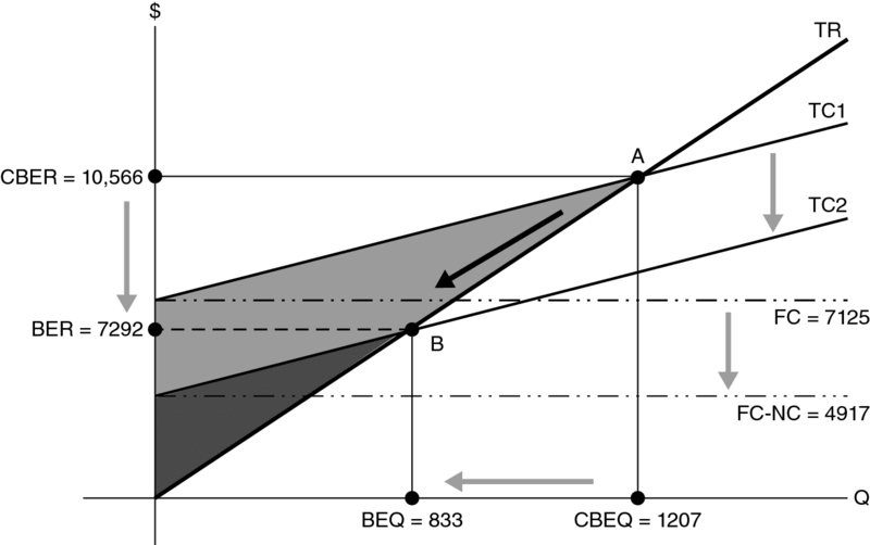
Figure 8.7 Break-even Point and Shifts in Cost
The last word about the cost–value–profit or break-even analysis is that it is a simple but important business analysis that offers a clearer view of the relationship between operating cost, revenue, and profits. Many firms can use it in an even more simplified version to assess their firm's status of sales and profits. One of these simplified applications is to translate the BEQ into a percentage of the firm's expected sales over a certain frame of time such as the first 2 or 5 years of the project operation. Such a percentage of sales can also be estimated in terms of its timing, hence having a much better perspective for the manager concerning how much work lies ahead and how tasks should be prioritized.
8.10 Profit Planning
Profit planning refers to the strategy, decisions, and procedures that a firm would take to ensure that its revenue would exceed all of its costs so that profits can be made. It includes a wide range of preparation and activities from a simple goal setting to budgeting to forecasting the future states of sales, revenues, and obligations. It would definitely require a heavy involvement by the manager and his team in order to translate their vision into tangible results that can be reaped in a specific frame of time and within the constraints of the firm's capabilities.
According to Walker and Petty (1986), profit plan constitutes a well-devised statement of goals, operating strategies, financial plans of action, and management information system. They further clear these requirements into the following three major elements:
- The firm's objectives as set forth by the owners.
- The avenues for achieving these objectives.
- A system for providing continuous feedback to the organization's progress in reaching these objectives.
To efficiently achieve these goals, an operating plan would provide order and explanation of the action to be taken during the planning horizon, especially in identifying the productive alternatives and estimating their costs and revenues and selecting the best feasible alternative that would fit the established objectives. As this operating plan should lead to realizing the expected profit, a financial plan would detail the steps to guide the firm's finances toward that goal. The financial plan would project capital investment and anticipate earnings, set cash budget, and complete pro forma profit and loss as well as pro forma balance sheet. Finally, the management information system would help evaluate the results and assess them against the benchmarks. The assessment of what has been achieved in comparison to the goals and the pre-established benchmarks may be done in short intervals in order to take advantage of the right opportunity to modify methods and approaches and take corrective actions that could be much easier to apply instead of waiting for the end of the horizon plan. Although firms are different in their philosophies and methods, we can be sure that all would need to have a great knowledge of their cost and revenue in order to draw a sensible profit plan. This would most certainly involve forecasting sales of products to estimate revenue as well as forecasting the production costs. The forecast methods and procedures will be detailed in Chapter 9.
8.11 Summary
This chapter addressed the profit as a concept and as a practical measure for business. It also went over the cost–volume analysis which would theoretically determine when a business would start to collect profits. The chapter started off by distinguishing between the two common concepts of profit, the accounting and economics concepts. Then came the explanation of the profit margin and markup with math formulas and numerical examples. Profit and cash flow were next to be clarified with the help of a comprehensive diagram. This was followed by a discussion on profitability and earning power.
The second part of the chapter started with the question, “When would a firm start collecting profits?” The answer required a detailed explanation of the cost–value analysis. With math, graphs, and numerical examples, the topic of the break-even analysis was addressed comprehensively. It went over how to get the BEQ of a product, the BER in dollars, the contribution margin, and the separation between fixed and variable costs that is required for the calculation of both the constructs, BEQ and BER. Using the cost–volume analysis enabled us to obtain the break-even point, in product and in dollars, if the entrepreneur decides in advance to obtain a certain profit. This profit was called the desired profit, and it could be added to the fixed cost to get the break-even point that would assure getting that profit after reaching the break-even point. Among the topics related to the cost–volume analysis was considering the non-cash charges in the calculation of the break-even point. The formula was adjusted by subtracting all the non-cash charges such as the depreciation from the fixed cost. Numerical examples were given, and graphs were showing the adjustment too.
Finally, the last topic in this chapter was profit planning, which refers to all strategies, and procedures that a firm would follow in order to assure obtaining a positive profit.
Key Concepts
- Accountant's profit
-
Economist's profit Cost–volume analysis
- Explicit cost
-
Implicit cost Markup
- Gross profit margin
-
Net profit margin Retailer's cost
- Cash inflow
-
Cash outflow Profitability
- Earning power
-
Total asset turnover Break-even point
- Break-even analysis
-
Break-even quantity Break-even revenue
- Cost–volume–profit analysis
-
Fixed cost
- Variable cost
-
Contribution margin Non-cash charges
- Profit planning
Discussion Questions
-
What is the difference between an accountant's profit and an economist's profit?
-
What is the difference between profit margin and markup?
-
Is the markup a percent out of the retailer's cost or the retail price? Illustrate your answers with a numerical example.
-
List at least four examples of each of the firm's cash inflow and its cash outflow.
-
What is profitability, and what is earning power? Prove mathematically that they are equal.
-
What is cost–volume–profit analysis? And how would it help the firm to figure out when it would start collecting profits?
-
Define both the break-even quantity and the break-even revenue and provide their formulas.
-
What is the break-even point? Define it conceptually, mathematically, and graphically.
-
Can an entrepreneur set his desired profit? And how would he do that technically?
-
How could the non-cash cost such as the depreciation be considered if you want to find out the break-even point? Explain that with a numerical example.