APPENDIX A
Informal Definitions of Statistical Terms
ALL KINDS OF PHENOMENA are found to be distributed normally, that is, in the shape of a bell curve, shown in Figure A.1. For example, if we were to plot on a graph the number of eggs produced weekly by different hens, the number of errors occurring during production of a given type of automobile, or the IQ test scores for a group of people, the shape of the curve representing the data would approximate that of the bell curve. We do not need to go into the mathematical reasons for why distributions tend to have this shape. What is important is that the normal distribution curve has useful properties for making inferences about where observations stand in relation to other observations. The normal curve in Figure A.1 is divided into standard deviations—so named because the average score deviates from the mean by (approximately) this amount. In a perfectly normal distribution, which is a mathematical abstraction but one that is approximated surprisingly often if there are a very large number of observations, about 68 percent of all observations fall between +1 and –1 standard deviation (abbreviated SD) from the mean (set at 0 in the curve in Figure A.1). Another set of useful facts about the concept of standard deviation concerns the relation between percentiles and standard deviations. About 84 percent of all observations occur at or below 1 SD above the mean; an observation at exactly 1 SD above the mean is at the 84th percentile of the distribution. Sixteen percent, the remaining observations, occur above that standard deviation. Almost 98 percent of all observations lie below 2 SDs above the mean. A score at exactly 2+ SDs from the mean is at the 98th percentile. The remaining 2 percent of observations are above that. Nearly all observations fall between 3 SDs below the mean and 3 SDs above it. By convention, the SD of the distribution of scores on most IQ tests is forced to be 15 (with a mean of 100).
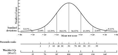
Figure A.1. The normal distribution curve, with standard deviations from the mean marked by vertical lines and with corresponding percentile scores and Wechsler IQ scores given below. Note that 68 percent of values fall between 1 standard deviation (σ) below the mean and 1 standard deviation above the mean.
Standard deviations are useful units with which to describe effect sizes, for example, in determining how much difference a new teaching technique makes to what the students learn. The most common indicator of effect size is a statistic called Cohen’s d, which is calculated as follows: the mean of group A minus the mean of group B divided by the average of the standard deviations of the two groups (or sometimes divided by the standard deviation just of group A).
By convention, d values of .20 or less are deemed small. This is the equivalent of moving the experimental group’s scores from the 50th percentile to almost the 60th percentile. You might not think that was such a small effect if the scores in question were those that could be expected by your child if he or she is taught by the new technique (60th percentile) versus the old technique (50th percentile). And whether you would be willing to pay for the technique depends in part on how important the difference between the 50th percentile and 60th percentile is. If you are measuring teaching effectiveness in terms of how quickly a child learns the touch typing system to a proficiency of 40 words per minute, and the difference between the 50th and 60th percentiles amounts to a few days, you probably would not be willing to pay too much for that gain and would not want your school system to pay much for it either. If you are comparing the effectiveness of two high school math teaching techniques by looking at average scores on the SAT exam, and one technique results in an average score of 500 and the other results in an average score of 520, this is the difference between the 50th and the 60th percentiles (assuming that the SD of SAT scores is 100). You might be willing to pay some significant amount of money for it. And you might be happy if your school board paid a modest amount per pupil to spring for the more effective method.
By convention, d values of .50 or so are considered moderate. In the world of IQ tests and academic achievement, though, an effect size of that magnitude would normally be considered a bombshell. It is the difference between an SAT score on the math section of 500 and one of 550—sometimes enough to make the difference between being accepted to a fairly good university and a significantly better university. You and your school system might be willing to pay a considerable amount to adopt a new method that would move the average child from the 50th percentile of SAT math scores to about the 70th percentile (which is what .50 SD corresponds to).
Effect sizes in the range of .70 to 1.00 SD are considered large. For education or intelligence differences, an effect size of 1.00 is huge. The putative IQ difference between blacks and whites is on the order of 1.00 SD. In Chapter 6, I discussed whether that is the actual magnitude of the difference. If it were, it would mean that the average IQ for blacks stood at the 16th percentile of the distribution of IQs for whites. An intervention that took children from, on average, the 50th percentile of the national distribution in math achievement scores to the 84th percentile would be considered worth it even at very great cost. For a nation, the increase in competitiveness that could result from such an improvement in math scores would be worth an enormous economic outlay.
The correlation coefficient is a measure of the degree of linear association between two variables. For example, the correlation between IQ scores and academic grades happens to fall around .50, indicating a moderately high degree of association. At least a moderate association should be expected because IQ tests were invented to predict how well people would do in school. Correlation coefficients range between –1, indicating a perfect negative association, and +1, indicating a perfect positive association. A correlation coefficient of 0 indicates no association at all. The correlation coefficient is another measure of effect size or, rather, of relationship magnitude, with values lower than .30 considered to be small, values of .30 to .50 considered moderate, and values above .50 considered to be large. But, as with effect size, whether a correlation is important or not has more to do with the variables represented in the correlation than with the size of the correlation. The correlation coefficient is interpretable in standard deviation terms. A correlation of .25 between two variables indicates that an increase of 1 SD in the first variable is associated with an increase of .25 SD in the second variable; a correlation of .50 is associated with an increase of .50 SD. So if the correlation between class size and student achievement on a standardized test were ®.25, then a decrease of class size by 1 SD could be expected to produce an improvement in test scores of .25 SD (assuming that the relationship between class size and test scores is genuinely a causal one).
Multiple regression is a way of simultaneously correlating a number of independent or predictor variables with some target or outcome variable. For example, we might want to compare the degree to which a number of variables predict the appeal of houses on the real estate market. We might measure the area in square feet, the number of bedrooms, the opulence of the master bathroom (for example, using an index based on the number of sinks, the presence or absence of a hot tub, and the use of high-or low-quality materials), the average income in the neighborhood, and the charm of the house as rated by a panel of potential buyers. We then correlate each of these variables simultaneously with the appeal of the house as measured by the amount that it can fetch on the market—the target variable. We get an estimate of the contribution of a given variable to the market value by finding out the size of the correlation of the variable with market value net of the contribution of all the other variables (that is, holding all other variables constant). Thus, charm, holding all other variables constant, might be correlated .25 with market value, and master bath opulence might be correlated .10 with market value. But all of the variables are going to be correlated with one another, and some of the variables are measured with greater precision than others, and some of the variables have a causal relation with others while others do not, and some variables that have not been measured are going to exert an effect on some of those that have been measured. The result is that multiple-regression analysis can mislead us. The actual magnitude of the contribution of charm to market price could be substantially higher or lower than the figure of .25 derived from the regression analysis.
There are endless numbers of instances where multiple-regression analysis gives one impression about causality and actual experiments, which are nearly always greatly preferable from the standpoint of causal inference, give another. For example, about fifteen years ago, I attended a consensus development conference put on by the National Institutes of Health. The purpose of the conference was to review research on medical procedures versus surgical procedures as treatments for coronary artery blockage and reach consensus about the appropriateness of each. The results of a very large number of expensive American studies, paid for by government funds, were available. In those studies, researchers put a host of variables about patients such as illness history, age, and socioeconomic status (SES) into a multiple-regression equation and drew conclusions about the effect of treatment type “net” of all the other ways in which patients varied. But because Internal Review Boards governing research policy in the United States require allowing patients to choose their treatment (it is far from clear that this is actually in the patients’ interests), all the U.S. evidence was undermined by the self-selection artifact (see below). But in addition to the American studies were two European studies based on the random assignment of patients to treatment. Quite correctly, the panelists ignored the expensive American studies and considered only the results of the European studies.
Let’s consider an example closer to the topic of this book, namely, whether size of class matters to student performance. Multiple-regression analysis tells us that, net of size of school, and average income of families in the neighborhood where the school is located, and teacher salary, and percentage of teachers who are certified, and amount of money spent per pupil in the district, and so on, average class size is uncorrelated with student performance (Hanushek, 1986; Hoxby, 2000; Jencks et al., 1972). But one well-conducted, randomized experiment varying class size over a substantial amount (13 to 17 pupils per class as compared to 22 to 25 pupils per class) found that class size varied to that degree produces an improvement in standardized test performance of more than .25 SD—and the effect on black children was greater than the effect on white children (Krueger, 1999). This was not merely another study on the effects of class size. It replaced all the multiple-regression studies on class size.
I occasionally cite multiple-regression studies in this book, but sparingly and always with a warning to beware the results.
Self-selection is one of the problems underlying the difficulty of interpreting correlational studies and multiple-regression analyses, and it is crucial to understand, for many reasons. When we say that IQ is correlated with occupational success to a particular degree—say, .40—there is a reflexive tendency to assume that the relationship is entirely causal: higher IQ makes a person perform a job better. But IQ is correlated with other factors too. For example, higher IQ in a child is associated with higher SES of that child’s parents, which, for example, makes it more likely that the child will go to college regardless of the child’s IQ level. And a college education, again regardless of IQ level, makes higher occupational status more likely. Thus, the correlation between IQ and occupational success is contaminated by the contribution of other variables like parents’ SES and college attendance, which the child, or subject, has been allowed to “self-select.” (It is odd to say that a person “self-selects” for something like parents’ SES, which the person obviously did not choose. But the comparison is with the investigator, who clearly did not determine the level for that variable, so it is as if the person determined the level. At any rate, something about the person that the investigator had no control over was allowed to vary without the investigator’s selection, or even knowledge, of the person’s level on the variable.)
Any time a study merely measures, as opposed to manipulates, a given variable, we have to recognize that the subject and not the investigator has selected the level of the variable in question—along with the levels on all other variables measured or not. This gives up a huge degree of inferential power. In the class-size example, the investigator using multiple regression has allowed the level on the class-size variable to be self-selected (that is, the investigator did not determine class size), and the class-size variable may be associated with all sorts of other variables that may amplify or block the effects of class size on achievement. The only way to completely avoid the self-selection problem is for the investigator to select the value on the independent or predictor variable (for example, big class versus small class) and then observe its effects on the target variable (for example, achievement test performance). Alas, this is not always possible, so we have to be content with correlational analyses and multiple-regression analyses, hedged with caveats about the self-selection problem.
Finally, statistical significance tells us the likelihood that a result—for example, an effect of class size on performance—could have occurred by chance if the true effect is actually zero. The conventional value for statistical significance is .05, meaning that a difference between two means, or a correlation of a given size, would occur by chance only 5 in 100 times, or 1 in 20 times, in a study having the same design as the study in question. Statistical significance is very much a function of the number of observations. Even differences so small as to be of no practical or theoretical significance can be statistically significant if there are enough observations. Every result based on a study that I report in this book is statistically significant at least at the .05 level, except in one instance where I report a result that is “marginally significant,” with a probability of less than .10 that the result would have been obtained by chance.