In addressing any problem in continuum or solid mechanics, three factors must be considered: (1) the Newtonian equations of motion, in the more general form recognized by Euler, expressing conservation of linear and angular momentum for finite bodies (rather than just for point particles), and the related concept of stress, as formalized by Cauchy, (2) the geometry of deformation and thus the expression of strains in terms of gradients in the displacement field, and (3) the relations between stress and strain that are characteristic of the material in question, as well as of the stress level, temperature, and time scale of the problem considered.
These three considerations suffice for most problems. They must be supplemented, however, for solids undergoing diffusion processes in which one material constituent moves relative to another (which may be the case for fluid-infiltrated soils or petroleum reservoir rocks) and in cases for which the induction of a temperature field by deformation processes and the related heat transfer cannot be neglected. These cases require that the following also be considered: (4) equations for conservation of mass of diffusing constituents, (5) the first law of thermodynamics, which introduces the concept of heat flux and relates changes in energy to work and heat supply, and (6) relations that express the diffusive fluxes and heat flow in terms of spatial gradients of appropriate chemical potentials and of temperature. In many important technological devices, electric and magnetic fields affect the stressing, deformation, and motion of matter. Examples are provided by piezoelectric crystals and other ceramics for electric or magnetic actuators and by the coils and supporting structures of powerful electromagnets. In these cases, two more considerations must be added: (7) James Clerk Maxwell’s set of equations interrelating electric and magnetic fields to polarization and magnetization of material media and to the density and motion of electric charge, and (8) augmented relations between stress and strain, which now, for example, express all of stress, polarization, and magnetization in terms of strain, electric field, magnetic intensity, and temperature. The second law of thermodynamics, combined with the above-mentioned principles, serves to constrain physically allowed relations between stress, strain, and temperature in (3) and also constrains the other types of relations described in (6) and (8) above. Such expressions, which give the relationships between stress, deformation, and other variables, are commonly referred to as constitutive relations.
To examine the mathematical structure of the theory, considerations (1) to (3) above will now be further developed. For this purpose, a continuum model of matter will be used, with no detailed reference to its discrete structure at molecular—or possibly other larger microscopic—scales far below those of the intended application.
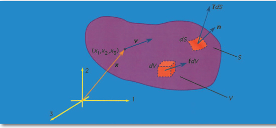
Let x denote the position vector of a point in space as measured relative to the origin of a Newtonian reference frame; x has the components (x1, x2, x3) relative to a Cartesian set of axes, which is fixed in the reference frame and denoted as the 1, 2, and 3 axes. Suppose that a material occupies the part of space considered, and let υ = υ (x, t) be the velocity vector of the material point that occupies position x at time t; that same material point will be at position x + υdt an infinitesimal interval dt later. Let ρ = ρ (x, t) be the mass density of the material. Here υ and ρ are macroscopic variables. What is idealized in the continuum model as a material point, moving as a smooth function of time, will correspond on molecular-length (or larger but still “microscopic”) scales to a region with strong fluctuations of density and velocity. In terms of phenomena at such scales, ρ corresponds to an average of mass per unit of volume, and ρυ to an average of linear momentum per unit volume, as taken over spatial and temporal scales that are large compared to those of the microscale processes but still small compared to those of the intended application or phenomenon under study. Thus, from the microscopic viewpoint, υ of the continuum theory is a mass-weighted average velocity.
The position vector x and the velocity vector υ of a material point, the body force fdV acting on an element dV of volume, and the surface force TdS acting on an element dS of surface in a Cartesian coordinate system 1, 2, 3. Copyright Encyclopædia Britannica; rendering for this edition by Rosen Educational Services
The linear momentum P and angular momentum H (relative to the coordinate origin) of the matter instantaneously occupying any volume V of space are then given by summing up the linear and angular momentum vectors of each element of material. Such summation over infinitesimal elements is represented mathematically by the integrals P = ∫νρυdV and H = ∫νρx × υdV. In this discussion attention is limited to situations in which relativistic effects can be ignored. Let F denote the total force and M the total torque, or moment (relative to the coordinate origin), acting instantaneously on the material occupying any arbitrary volume V. The basic laws of Newtonian mechanics are the linear and angular momentum principles that F = dP/dt and M = dH/dt, where time derivatives of P and H are calculated following the motion of the matter that occupies V at time t. When either F or M vanishes, these equations of motion correspond to conservation of linear or angular momentum.
An important, very common, and nontrivial class of problems in solid mechanics involves determining the deformed and stressed configuration of solids or structures that are in static equilibrium; in that case the relevant basic equations are F = 0 and M = 0. The understanding of such conditions for equilibrium, at least in a rudimentary form, long predates Newton. Indeed, Archimedes of Syracuse (3rd century BCE), the great Greek mathematician and arguably the first theoretically and experimentally minded physical scientist, understood these equations at least in a nonvectorial form appropriate for systems of parallel forces. This is shown by his treatment of the hydrostatic equilibrium of a partially submerged body and by his establishment of the principle of the lever (torques about the fulcrum sum to zero) and the concept of centre of gravity.
Assume that F and M derive from two types of forces, namely, body forces f, such as gravitational attractions—defined such that force fdV acts on volume element dV—and surface forces, which represent the mechanical effect of matter immediately adjoining that along the surface S of the volume V being considered. Cauchy formalized in 1822 a basic assumption of continuum mechanics that such surface forces could be represented as a stress vector T, defined so that TdS is an element of force acting over the area dS of the surface. Hence, the principles of linear and angular momentum take the forms
which are now assumed to hold good for every conceivable choice of region V. In calculating the right-hand sides, which come from dP/dt and dH/dt, it has been noted that ρdV is an element of mass and is therefore time-invariant; also, a = a(x, t) = dυ/dt is the acceleration, where the time derivative of υ is taken following the motion of a material point so that a (x, t) dt corresponds to the difference between υ(x + υdt, t + dt) and υ (x, t). A more detailed analysis of this step shows that the understanding of what TdS denotes must now be adjusted to include averages, over temporal and spatial scales that are large compared to those of microscale fluctuations, of transfers of momentum across the surface S due to the microscopic fluctuations about the motion described by the macroscopic velocity υ.
The nine components of a stress tensor. The first index denotes the direction of the normal, or perpendicular, stresses to the plane across which the contact force acts, and the second index denotes the direction of the component of force. Copyright Encyclopædia Britannica; rendering for this edition by Rosen Educational Services
The nine quantities σij (i, j = 1, 2, 3) are called stress components; these will vary with position and time—i.e., σij = σij(x, t)—and have the following interpretation. Consider an element of surface dS through a point x with dS oriented so that its outer normal (pointing away from the region V, bounded by S) points in the positive xi direction, where i is any of 1, 2, or 3. Then σi1, σi2, and σi3 at x are defined as the Cartesian components of the stress vector T (called T(i)) acting on this dS. To use a vector notation with e1, e2, and e3 denoting unit vectors along the coordinate axes, T(i) = σi1 e1 + σi2 e2 + σi3 e3. Thus, the stress σij at x is the stress in the j direction associated with an i-oriented face through point x; the physical dimension of the σij is [force]/[length]2. The components σ11, σ22, and σ33 are stresses directed perpendicular, or normal, to the face on which they act and are normal stresses; the σij with i ≠ j are directed parallel to the face on which they act and are shear stresses.
The force TdS acting on an arbitrarily inclined face (whose outward unit normal vector is n). Stress vectors T(-1) T(-2), and T(-3) act on the faces perpendicular to the coordinate axes. Copyright Encyclopædia Britannica; rendering for this edition by Rosen Educational Services
By hypothesis, the linear momentum principle applies for any volume V. Consider a small tetrahedron at x with an inclined face having an outward unit normal vector n and its other three faces oriented perpendicular to the three coordinate axes. Letting the size of the tetrahedron shrink to zero, the linear momentum principle requires that the stress vector T on a surface element with outward normal n be expressed as a linear function of the σij at x. The relation is such that the j component of the stress vector T is Tj = n1σ1j + n2 σ2j + n3σ3j for (j = 1, 2, 3). This relation for (j = 1, 2, 3). This relation for T (or Tj) also demonstrates that the σij have the mathematical property of being the components of a second-rank tensor.
Suppose that a different set of Cartesian reference axes 1′, 2′, and 3′ have been chosen. Let ![]() ,
, ![]() , and
, and ![]() denote the components of the position vector of point x and let
denote the components of the position vector of point x and let ![]() denote the nine stress components relative to that coordinate system. The
denote the nine stress components relative to that coordinate system. The ![]() can be written as the 3 × 3 matrix [σ′], and the σij as the matrix [σ], where the first index is the matrix row number and the second is the column number. Then the expression for Tj implies that [σ′] = [α][σ][α]T, which is the defining equation of a second-rank tensor. Here [α] is the orthogonal transformation matrix, having components
can be written as the 3 × 3 matrix [σ′], and the σij as the matrix [σ], where the first index is the matrix row number and the second is the column number. Then the expression for Tj implies that [σ′] = [α][σ][α]T, which is the defining equation of a second-rank tensor. Here [α] is the orthogonal transformation matrix, having components ![]() for p, q = 1, 2, 3 and satisfying [α]T [α] = [α][α]T = [I], where the superscript T denotes transpose (interchange rows and columns) and [I] denotes the unit matrix, a 3 × 3 matrix with unity for every diagonal element and zero elsewhere; also, the matrix multiplications are such that if [A] = [B][C], then Aij = Bi1 C1j + Bi2 C2j + Bi3 + C3j.
for p, q = 1, 2, 3 and satisfying [α]T [α] = [α][α]T = [I], where the superscript T denotes transpose (interchange rows and columns) and [I] denotes the unit matrix, a 3 × 3 matrix with unity for every diagonal element and zero elsewhere; also, the matrix multiplications are such that if [A] = [B][C], then Aij = Bi1 C1j + Bi2 C2j + Bi3 + C3j.
Now the linear momentum principle may be applied to an arbitrary finite body. Using the expression for Tj above and the divergence theorem of multivariable calculus, which states that integrals over the area of a closed surface S, with integrand nif(x), may be rewritten as integrals over the volume V enclosed by S, with integrand ∂f(x)/∂xi; when f(x) is a differentiable function, one may derive that
![]()
at least when the σij are continuous and differentiable, which is the typical case. These are the equations of motion for a continuum. Once the above consequences of the linear momentum principle are accepted, the only further result that can be derived from the angular momentum principle is that σij = σji (i, j = 1, 2, 3). Thus, the stress tensor is symmetric.
Symmetry of the stress tensor has the important consequence that, at each point x, there exist three mutually perpendicular directions along which there are no shear stresses. These directions are called the principal stress directions, and the corresponding normal stresses are called the principal stresses. If the principal stresses are ordered algebraically as σI, σII, and σIII, then the normal stress on any face (given as σn = n · T) satisfies σI ≤ σn ≤ σIII. The principal stresses are the eigenvalues (or characteristic values) s, and the principal directions the eigenvectors n, of the problem T = sn, or [σ]{n} = s{n} in matrix notation with the 3-column {n} representing n. It has solutions when det ([σ] - s[I]) = - s3 + I1s2 + I2s + I3 = 0, with I1 = tr[σ], I2 = -(1/2)I 2/1 + (1/2)tr([σ][σ]), and I3 = det [σ]. Here “det” denotes determinant and “tr” denotes trace, or sum of diagonal elements, of a matrix. Since the principal stresses are determined by I1, I2, and I3 and can have no dependence on how one chooses the coordinate system with respect to which the components of stress are referred, I1, I2, and I3 must be independent of that choice and are therefore called stress invariants. One may readily verify that they have the same values when evaluated in terms of σij′ above as in terms of σij by using the tensor transformation law and properties noted for the orthogonal transformation matrix.
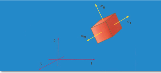
Principal stresses. Copyright Encyclopædia Britannica; rendering for this edition by Rosen Educational Services
Very often, in both nature and technology, there is interest in structural elements in forms that might be identified as strings, wires, rods, bars, beams, or columns, or as membranes, plates, or shells. These are usually idealized as, respectively, one- or two-dimensional continua. One possible approach is then to develop the consequences of the linear and angular momentum principles entirely within that idealization, working in terms of net axial and shear forces and bending and twisting torques at each point along a one-dimensional continuum, or in terms of forces and torques per unit length of surface in a two-dimensional continuum.
The shape of a solid or structure changes with time during a deformation process. To characterize deformation, or strain, a certain reference configuration is adopted and called undeformed. Often, that reference configuration is chosen as an unstressed state, but such is neither necessary nor always convenient. If time is measured from zero at a moment when the body exists in that reference configuration, then the upper case X may be used to denote the position vectors of material points when t = 0. At some other time t, a material point that was at X will have moved to some spatial position x. The deformation is thus described as the mapping x = x(X, t), with x = x(X, 0) = X. The displacement vector u is then u = x(X, t) - X; also, υ = ∂x(X, t)/∂t and a = ∂2x(X, t)/∂t2.
It is simplest to write equations for strain in a form that, while approximate in general, is suitable for the case when any infinitesimal line element dX of the reference configuration undergoes extremely small rotations and fractional change in length, in deforming to the corresponding line element dx. These conditions are met when | ∂ui/∂Xj| << 1. Many solids are often sufficiently rigid, at least under the loadings typically applied to them, that these conditions are realized in practice. Linearized expressions for strain in terms of [∂u/∂X], appropriate to this situation, are called small strain or infinitesimal strain. Expressions for strain will also be given that are valid for rotations and fractional length changes of arbitrary magnitude; such expressions are called finite strain.
Two simple types of strain are extensional strain and shear strain. Consider a rectangular parallelepiped, a bricklike block of material with mutually perpendicular planar faces, and let the edges of the block be parallel to the 1, 2, and 3 axes. If the block is deformed homogeneously, so that each planar face moves perpendicular to itself and so that the faces remain orthogonal (i.e., the parallelepiped is deformed into another rectangular parallelepiped), then the block is said to have undergone extensional strain relative to each of the 1, 2, and 3 axes but no shear strain relative to these axes. If the edge lengths of the undeformed parallelepiped are denoted as ΔX1, ΔX2, and ΔX3, and those of the deformed parallelepiped as Δx1, Δx2, and Δx3, then the quantities λ1 = Δx1/ΔX1, λ2 = Δx2/ΔX2, and λ = Δx3/ΔX3 are called stretch ratios. There are various ways that extensional strain can be defined in terms of them. Note that the change in displacement in, say, the x1 direction between points at one end of the block and those at the other is Δu1 = (λ1 - 1)ΔX1. For example, if E11 denotes the extensional strain along the x1 direction, then the most commonly understood definition of strain is E11 = (change in length)/(initial length) = (Δx1 - ΔX1)/ΔX1 = Δu1/ΔX1 = λ1 - 1. A variety of other measures of extensional strain can be defined by E11 = g(λ1), where the function g(λ) satisfies g(1) = 0 and g′(1) = 1, so as to agree with the above definition when λ1 is very near 1. Two such measures in common use are the strain ![]() , based on the change of metric tensor, and the logarithmic strain E L = ln(λ1).
, based on the change of metric tensor, and the logarithmic strain E L = ln(λ1).

(A) extensional strain and (B) simple shear strain, where the element drawn with dashed lines represents the reference configuration, and the element drawn with solid lines represents the deformed configuration. Copyright Encyclopædia Britannica; rendering for this edition by Rosen Educational Services
To define a simple shear strain, consider the same rectangular parallelepiped, but now deform it so that every point on a plane of type X2 = constant moves only in the x1 direction by an amount that increases linearly with X2. Thus, the deformation x1 = γX2 + X1, x2 = X2, x3 = X3 defines a homogeneous simple shear strain of amount γ. Note that this strain causes no change of volume. For small strain, the shear strain γ can be identified as the reduction in angle between two initially perpendicular lines.
The small strains, or infinitesimal strains, εij are appropriate for situations with |∂uk/∂X1| << I for all k and l. Consider two infinitesimal material fibres, one initially in the 1 direction and the other in the 2 direction. To first-order accuracy in components of [∂u/∂X], the extensional strains of these fibres are ε11 = ∂u1/∂X1 and ε22 = ∂u2/∂X2, and the reduction of the angle between them is γ 12 = ∂u2/∂X1 + ∂u1/∂X2. For the shear strain denoted ε12, however, half of γ12 is used. Thus, considering all extensional and shear strains associated with infinitesimal fibres in the 1, 2, and 3 directions at a point of the material, the set of strains is given by

Relations of strains to gradients of displacement. Copyright Encyclopædia Britannica; rendering for this edition by Rosen Educational Services
The εij are symmetric—i.e., εij = εji—and form a second-rank tensor (that is, if Cartesian reference axes 1′, 2′, and 3′ were chosen instead and the εkl′ were determined, then the εkl′ are related to the εij by the same equations that relate the stresses σkl′ to the σij). These mathematical features require that there exist principal strain directions; at every point of the continuum it is possible to identify three mutually perpendicular directions along which there is purely extensional strain, with no shear strain between these special directions. The directions are the principal strain directions, and the corresponding strains include the least and greatest extensional strains experienced by fibres through the material point considered. Invariants of the strain tensor may be defined in a way paralleling those for the stress tensor.
An important fact to note is that the strains cannot vary in an arbitrary manner from point to point in the body. This is because the six strain components are all derivable from three displacement components. Restrictions on strain resulting from such considerations are called compatibility relations; the body would not fit together after deformation unless they were satisfied. Consider, for example, a state of plane strain in the 1, 2 plane (so that ε33 = ε23 = ε31 = 0). The nonzero strains ε11, ε22, and ε12 cannot vary arbitrarily from point to point but must satisfy ![]() , as may be verified by directly inserting the relations for strains in terms of displacements.
, as may be verified by directly inserting the relations for strains in terms of displacements.
When the smallness of stretch and rotation of line elements allows use of the infinitesimal strain tensor, a derivative ∂/∂Xi will be very nearly identical to ∂/∂xi. Frequently, but not always, it will then be acceptable to ignore the distinction between the deformed and undeformed configurations in writing the governing equations of solid mechanics. For example, the differential equations of motion in terms of stress are rigorously correct only with derivatives relative to the deformed configuration, but, in the circumstances considered, the equations of motion can be written relative to the undeformed configuration. This is what is done in the most widely used variant of solid mechanics, in the form of the theory of linear elasticity. The procedure can be unsatisfactory and go badly wrong in some important cases, however, such as for columns that buckle under compressive loadings or for elastic-plastic materials when the slope of the stress versus strain relation is of the same order as existing stresses. Cases such as these are instead best approached through finite deformation theory.
In the theory of finite deformations, extension and rotations of line elements are unrestricted as to size. For an infinitesimal fibre that deforms from an initial point given by the vector dX to the vector dx in the time t, the deformation gradient is defined by Fij = ∂xi(X, t)/∂Xj; the 3 × 3 matrix [F], with components Fij, may be represented as a pure deformation, characterized by a symmetric matrix [U], followed by a rigid rotation [R]. This result is called the polar decomposition theorem and takes the form, in matrix notation, [F] = [R][U]. For an arbitrary deformation, there exist three mutually orthogonal principal stretch directions at each point of the material; call these directions in the reference configuration N(I), N(II), N(III), and let the stretch ratios be λI, λII, λIII. Fibres in these three principal strain directions undergo extensional strain but have no shearing between them. Those three fibres in the deformed configuration remain orthogonal but are rotated by the operation [R].
As noted earlier, an extensional strain may be defined by E = g(λ), where g(1) = 0 and g′(1) = 1, with examples for g(λ) given above. A finite strain tensor Eij may then be defined based on any particular function g(λ) by Eij = g(λ1) Ni(I) Nj(I) + g(λII) Ni(II) Nj(II) + g(λIII) Ni(III) Nj(III). Usually, it is rather difficult to actually solve for the λ’s and N’s associated with any general [F], so it is not easy to use this strain definition. However, for the special choice identified as gM(λ) = (λ2 - 1)/2 above, it may be shown that
![]()
which, like the finite strain generated by any other g(λ), reduces to εij when linearized in [∂u/∂X].
In general, the stress-strain relations are to be determined by experiment. A variety of mechanical testing machines and geometric configurations of material specimens have been devised to measure them. These allow, in different cases, simple tensile, compressive, or shear stressing, and sometimes combined stressing with several different components of stress, as well as the determination of material response over a range of temperatures, strain rates, and loading histories. The testing of round bars under tensile stress, with precise measurement of their extension to obtain the strain, is common for metals and for technological ceramics and polymers. For rocks and soils, which generally carry load in compression, the most common test involves a round cylinder that is compressed along its axis, often while being subjected to confining pressure on its curved face. Frequently, a measurement interpreted by solid mechanics theory is used to determine some of the properties entering stress-strain relations. For example, measuring the speed of deformation waves or the natural frequencies of vibration of structures can be used to extract the elastic moduli of materials of known mass density, and measurement of indentation hardness of a metal can be used to estimate its plastic shear strength.
In some favourable cases, stress-strain relations can be calculated approximately by applying principles of mechanics at the microscale of the material considered. In a composite material, the microscale could be regarded as the scale of the separate materials making up the reinforcing fibres and matrix. When their individual stress-strain relations are known from experiment, continuum mechanics principles applied at the scale of the individual constituents can be used to predict the overall stress-strain relations for the composite. For rubbery polymer materials, made up of long chain molecules that randomly configure themselves into coil-like shapes, some aspects of the elastic stress-strain response can be obtained by applying principles of statistical thermodynamics to the partial uncoiling of the array of molecules by imposed strain. For a single crystallite of an element such as silicon or aluminum or for a simple compound like silicon carbide, the relevant microscale is that of the atomic spacing in the crystals; quantum mechanical principles governing atomic force laws at that scale can be used to estimate elastic constants. In the case of plastic flow processes in metals and in sufficiently hot ceramics, the relevant microscale involves the network of dislocation lines that move within crystals. These lines shift atom positions relative to one another by one atomic spacing as they move along slip planes. Important features of elastic-plastic and viscoplastic stress-strain relations can be understood by modeling the stress dependence of dislocation generation and motion and the resulting dislocation entanglement and immobilization processes that account for strain hardening.
The simplest type of stress-strain relation is that of the linear elastic solid, considered in circumstances for which |∂ui/∂Xj|<< 1 and for isotropic materials, whose mechanical response is independent of the direction of stressing. If a material point sustains a stress state σ11 = σ, with all other σij = 0, it is subjected to uniaxial tensile stress. This can be realized in a homogeneous bar loaded by an axial force. The resulting strain may be rewritten as ε11 = σ/E, ε22 = ε33 = -υε11 = -υσ/E,ε12 = ε23 = ε31 = 0. Two new parameters have been introduced here, E and υ. E is called Young’s modulus, and it has dimensions of [force]/[length]2 and is measured in units such as the pascal (1 Pa = 1 N/m2), dyne/cm2, or pounds per square inch (psi); υ, which equals the ratio of lateral strain to axial strain, is dimensionless and is called the Poisson ratio.
If the isotropic solid is subjected only to shear stress τ—i.e., σ12 = σ21 = τ, with all other σij = 0—then the response is shearing strain of the same type, ε12 = τ/2G, ε23 = ε31 = ε11 = ε22 = ε33 = 0. Notice that because 2ε12 = γ12, this is equivalent to γ12 = τ/G. The constant G introduced is called the shear modulus. (Frequently, the symbol μ is used instead of G.) The shear modulus G is not independent of E and υ but is related to them by G = E/2(1 + υ), as follows from the tensor nature of stress and strain. The general stress-strain relations are then
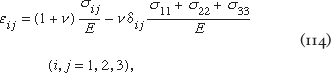
where δij is defined as I when its indices agree and 0 otherwise.
These relations can be inverted to read σij = λδij(ε11 + ε22 + ε33) + 2 μεij, where μ has been used rather than G as the notation for the shear modulus, following convention, and where λ = 2υμ/(1 - 2 υ). The elastic constants λand μ are sometimes called the Lamé constants. Since υ is typically in the range ¼ to ![]() for hard polycrystalline solids, λ falls often in the range between μ and 2μ. (Navier’s particle model with central forces leads to λ = μ for an isotropic solid.)
for hard polycrystalline solids, λ falls often in the range between μ and 2μ. (Navier’s particle model with central forces leads to λ = μ for an isotropic solid.)
Another elastic modulus often cited is the bulk modulus K, defined for a linear solid under pressure p(σ11 = σ22 = σ33 = - p) such that the fractional decrease in volume is p/K. For example, consider a small cube of side length L in the reference state. If the length along, say, the 1 direction changes to (1 + ε11)L, the fractional change of volume is (1 + ε11)(1 + ε22) (1 + ε33) - 1 = ε11 + ε22 + ε33, neglecting quadratic and cubic order terms in the εij compared to the linear, as is appropriate when using linear elasticity. Thus, K = E/3(1 - 2 υ) = λ+ 2μ/3.
Temperature change can also cause strain. In an isotropic material the thermally induced extensional strains are equal in all directions, and there are no shear strains. In the simplest cases, these thermal strains can be treated as being linear in the temperature change θ - θ0 (where θ0 is the temperature of the reference state), writing ![]() for the strain produced by temperature change in the absence of stress. Here α is called the coefficient of thermal expansion. Thus, in cases of temperature change, εij is replaced in the stress-strain relations above with
for the strain produced by temperature change in the absence of stress. Here α is called the coefficient of thermal expansion. Thus, in cases of temperature change, εij is replaced in the stress-strain relations above with ![]() , with the thermal part given as a function of temperature. Typically, when temperature changes are modest, the small dependence of E and υ on temperature can be neglected.
, with the thermal part given as a function of temperature. Typically, when temperature changes are modest, the small dependence of E and υ on temperature can be neglected.
Anisotropic solids also are common in nature and technology. Examples are single crystals; polycrystals in which the grains are not completely random in their crystallographic orientation but have a “texture,” typically owing to some plastic or creep flow process that has left a preferred grain orientation; fibrous biological materials such as wood or bone; and composite materials that, on a microscale, either have the structure of reinforcing fibres in a matrix, with fibres oriented in a single direction or in multiple directions (e.g., to ensure strength along more than a single direction), or have the structure of a lamination of thin layers of separate materials. In the most general case, the application of any of the six components of stress induces all six components of strain, and there is no shortage of elastic constants. There would seem to be 6 × 6 = 36 in the most general case, but, as a consequence of the laws of thermodynamics, the maximum number of independent elastic constants is 21 (compared with 2 for isotropic solids). In many cases of practical interest, symmetry considerations reduce the number to far below 21. For example, crystals of cubic symmetry, such as rock salt (NaCl); face-centred cubic metals, such as aluminum, copper, or gold; body-centred cubic metals, such as iron at low temperatures or tungsten; and such nonmetals as diamond, germanium, or silicon have only three independent elastic constants. Solids with a special direction, and with identical properties along any direction perpendicular to that direction, are called transversely isotropic; they have five independent elastic constants. Examples are provided by fibre-reinforced composite materials, with fibres that are randomly emplaced but aligned in a single direction in an isotropic or transversely isotropic matrix, and by single crystals of hexagonal close packing such as zinc.
General linear elastic stress-strain relations have the form

where the coefficients Cijkl are known as the tensor elastic moduli. Because the εkl are symmetric, one may choose Cijkl = Cijlk, and, because the σij are symmetric, Cijkl = Cjikl. Hence the 3 × 3 × 3 × 3 = 81 components of Cijkl reduce to the 6 × 6 = 36 mentioned. In cases of temperature change, the εij above is replaced by εij - εij thermal, where ε ijthermal = αij (θ - θ0) and αij is the set of thermal strain coefficients, with αij = αji. An alternative matrix notation is sometimes employed, especially in the literature on single crystals. That approach introduces 6-element columns of stress and strain {σ} and {ε}, defined so that the columns, when transposed (superscript T) or laid out as rows, are {σ}T = (σ11, σ22, σ33, σ12, σ23, σ31) and {ε}T = (ε11, ε22, ε33, 2ε12, 2ε23, 2ε31). These forms assure that the scalar {σ}T {dε} ≡ tr([σ][dε]) is an increment of stress working per unit volume. The stress-strain relations are then written {σ} = [c] {ε}, where [c] is the 6 × 6 matrix of elastic moduli. Thus, c 13 = C1133, c15 = C1123, c44 = C1212, and so on.
In thermodynamic terminology, a state of purely elastic material response corresponds to an equilibrium state, and a process during which there is purely elastic response corresponds to a sequence of equilibrium states and hence to a reversible process. The second law of thermodynamics assures that the heat absorbed per unit mass can be written θds, where θ is the thermodynamic (absolute) temperature and s is the entropy per unit mass. Hence, writing the work per unit volume of reference configuration in a manner appropriate to cases when infinitesimal strain can be used, and letting ρ0 be the density in that configuration, from the first law of thermodynamics it can be stated that ρ0θds + tr([σ][dε]) = ρ0de, where e is the internal energy per unit mass. This relation shows that if e is expressed as a function of entropy s and strains [ε], and if e is written so as to depend identically on εij and εji, then σij = ρ0∂e([ε], s)/∂εij.
Alternatively, one may introduce the Helmholtz free energy f per unit mass, where f = e -θs = f([ε], θ), and show that σij = ρ0∂f([ε], θ)/∂εij. The latter form corresponds to the variables with which the stress-strain relations were written above. Sometimes ρ0 f is called the strain energy for states of isothermal (constant θ) elastic deformation; ρ0e has the same interpretation for adiabatic (s = constant) elastic deformation, achieved when the time scale is too short to allow heat transfer to or from a deforming element. Since the mixed partial derivatives must be independent of order, a consequence of the last equation is that ∂σij([ε], θ)/∂εkl = ∂σkl([ε], θ)/∂εij, which requires that Cijkl = Cklij, or equivalently that the matrix [c] be symmetric, [c] = [c]T, reducing the maximum possible number of independent elastic constraints from 36 to 21. The strain energy W([ε]) at constant temperature θ0 is W([ε]) ≡ ρ0 f([ε], θ0) ≡ (½){ε}T[c]{ε}.
The elastic moduli for adiabatic response are slightly different from those for isothermal response. In the case of the isotropic material, it is convenient to give results in terms of G and K, the isothermal shear and bulk moduli. The adiabatic moduli G and K- are then G = G and K- = K(1 + 9θ0Kα2/ρ0cε), where cε = θ0∂s([ε],θ)/∂θ, evaluated at θ = θ0 and [ε] = [0], is the specific heat at constant strain. The fractional change in the bulk modulus, given by the second term in the parentheses, is very small, typically on the order of 1 percent or less, even for metals and ceramics of relatively high α, on the order of 10-5/kelvin.
The fractional change in absolute temperature during an adiabatic deformation is found to involve the same small parameter: [(θ - θ0)/θ0]s= const = -(9θ0Kα2/ρ0cε) [(ε11 + ε22 + ε33)/3αθ0]. Values of α for most solid elements and inorganic compounds are in the range of 10-6 to 4 × 10⁻⁵/kelvin; room temperature is about 300 kelvins, so 3αθ0 is typically in the range 10-3 to 4 × 10⁻². Thus, if the fractional change in volume is on the order of 1 percent, which is quite large for a metal or ceramic deforming in its elastic range, the fractional change in absolute temperature is also on the order of 1 percent. For those reasons, it is usually appropriate to neglect the alteration of the temperature field due to elastic deformation and hence to use purely mechanical formulations of elasticity in which distinctions between adiabatic and isothermal response are neglected.
When elastic response under arbitrary deformation gradients is considered—because rotations, if not strains, are large or, in a material such as rubber, because the strains are large too—it is necessary to dispense with the infinitesimal strain theory. In such cases, the combined first and second laws of thermodynamics have the form ρ0θds + det[F]tr([F]-1[σ][dF]) = ρ0de, where [F]-1 is the matrix inverse of the deformation gradient [F]. If a parcel of material is deformed by [F] and then given some additional rigid rotation, the free energy f must be unchanged in that rotation. In terms of the polar decomposition [F] = [R][U], this is equivalent to saying that f is independent of the rotation part [R] of [F], which is then equivalent to saying that f is a function of the finite strain measure [EM] = (½)([F]T[F] - [I]) based on change of metric or, for that matter, on any member of the family of material strain tensors. Thus,
is sometimes called the second Piola-Kirchhoff stress and is given by ![]() , it being assumed that f has been written so as to have identical dependence on
, it being assumed that f has been written so as to have identical dependence on ![]() and
and ![]() .
.
The above mode of expressing [σ] in terms of [S] is valid for solids showing viscoelastic or plastic response as well, except that [S] is then to be regarded not only as a function of the present [EM] and θ but also as dependent on the prior history of both. Assuming that such materials show elastic response to sudden stress changes or to small unloading from a plastically deforming state, [S] may still be expressed as a derivative of f, as above, but the derivative is understood as being taken with respect to an elastic variation of strain and is to be taken at fixed θ and with fixed prior inelastic deformation and temperature history. Such dependence on history is sometimes represented as a dependence of f on internal state variables whose laws of evolution are part of the inelastic constitutive description. There are also simpler models of inelastic response, and the most commonly employed forms for plasticity and creep in isotropic solids are presented next.
To a good approximation, plastic deformation of crystalline solids causes no change in volume; and hydrostatic changes in stress, amounting to equal change of all normal stresses, have no effect on plastic flow, at least for changes that are of the same order or magnitude as the strength of the solid in shear. Thus, plastic response is usually formulated in terms of deviatoric stress, which is defined by τij = σij - δij (σ11 + σ22 + σ33)/3. Following Richard von Mises, in a procedure that is found to agree moderately well with experiment, the plastic flow relation is formulated in terms of the second invariant of deviatoric stress, commonly rewritten as
![]()
and called the equivalent tensile stress. The definition is made so that, for a state of uniaxial tension, σ equals the tensile stress, and the stress-strain relation for general stress states is formulated in terms of data from the tensile test. In particular, a plastic strain εp in a uniaxial tension test is defined from εp = ε - σ/E, where ε is interpreted as the strain in the tensile test according to the logarithmic definition ε = lnλ, the elastic modulus E is assumed to remain unchanged with deformation, and σ/E << 1.
Thus, in the rate-independent plasticity version of the theory, tensile data (or compressive, with appropriate sign reversals) from a monotonic load test is assumed to define a function εp (σ). In the viscoplastic or high-temperature creep versions of the theory, tensile data is interpreted to define dεp/dt as a function of σ in the simplest case, representing, for example, secondary creep, and as a function of σ and εp in theories intended to represent transient creep effects or rate-sensitive response at lower temperatures. Consider first the rigid-plastic material model in which elastic deformability is ignored altogether, as is sometimes appropriate for problems of large plastic flow, as in metal forming or long-term creep in Earth’s mantle or for analysis of plastic collapse loads on structures. The rate of deformation tensor Dij is defined by 2Dij = ∂vi/∂xj + ∂vj/∂xi, and in the rigid-plastic case [D] can be equated to what may be considered its plastic part [Dp], given as ![]() . The numerical factors secure agreement between Dp11 and dεp/dt for uniaxial tension in the 1-direction. Also, the equation implies that
. The numerical factors secure agreement between Dp11 and dεp/dt for uniaxial tension in the 1-direction. Also, the equation implies that
![]()
which must be integrated over previous history to get εp as required for viscoplastic models in which dεp/dt is a function of σ and εp. In the rate-independent version, [Dp] is defined as zero whenever σ is less than the highest value that it has attained in the previous history or when the current value of σ is the highest value but dσ/dt < 0. (In the elastic-plastic context, this means that “unloading” involves only elastic response.) For the ideally plastic solid, which is idealized to be able to flow without increase of stress when σ equals the yield strength level, dεp/dt is regarded as an undetermined but necessarily nonnegative parameter, which can be determined (sometimes not uniquely) only through the complete solution of a solid mechanics boundary-value problem.
The elastic-plastic material model is then formulated by writing ![]() , where
, where ![]() is given in terms of stress and possibly stress rate as above and where the elastic deformation rates [De] are related to stresses by the usual linear elastic expression
is given in terms of stress and possibly stress rate as above and where the elastic deformation rates [De] are related to stresses by the usual linear elastic expression ![]() . Here the stress rates are expressed as the Jaumann co-rotational rates
. Here the stress rates are expressed as the Jaumann co-rotational rates
![]()
is a derivative following the motion of a material point and where the spin Ωij is defined by 2Ωij = ∂vi/∂xj - ∂vj/∂xi. The co-rotational stress rates are those calculated by an observer who spins with the average angular velocity of a material element. The elastic part of the stress-strain relation should be consistent with the existence of a free energy f, as discussed above. This is not strictly satisfied by the form just given, but the differences between it and one which is consistent in that way involves additional terms that are on the order of σ/E2 times the ![]() and are negligible in typical cases in which the theory is used, since σ/E is usually an extremely small fraction of unity, say, 10-4 to 10-2. A small-strain version of the theory is in common use for purposes of elastic-plastic stress analysis. In these cases, [D] is replaced with ∂ [ε(X, t)]/∂t, where [ε] is the small-strain tensor, ∂/∂x with ∂/∂X in all equations, and [σ*] with ∂[σ(X, t)]/∂t. The last two steps cannot always be justified, even in cases of very small strain when, for example, in a rate-independent material, dσ/dεp is not large compared to σ or when rates of rotation of material fibres can become much larger than rates of stretching, which is a concern for buckling problems even in purely elastic solids.
and are negligible in typical cases in which the theory is used, since σ/E is usually an extremely small fraction of unity, say, 10-4 to 10-2. A small-strain version of the theory is in common use for purposes of elastic-plastic stress analysis. In these cases, [D] is replaced with ∂ [ε(X, t)]/∂t, where [ε] is the small-strain tensor, ∂/∂x with ∂/∂X in all equations, and [σ*] with ∂[σ(X, t)]/∂t. The last two steps cannot always be justified, even in cases of very small strain when, for example, in a rate-independent material, dσ/dεp is not large compared to σ or when rates of rotation of material fibres can become much larger than rates of stretching, which is a concern for buckling problems even in purely elastic solids.
There are cases in which a deformed material body returns to its original shape and size when the forces causing the deformation are removed. A body with this ability is said to behave (or respond) elastically.
The final equations of the purely mechanical theory of linear elasticity (i.e., when coupling with the temperature field is neglected, or when either isothermal or isentropic response is assumed) are obtained as follows. The stress-strain relations are used, and the strains are written in terms of displacement gradients. The final expressions for stress are inserted into the equations of motion, replacing ∂/∂x with ∂/∂X in those equations. In the case of an isotropic and homogenous solid, these reduce to
![]()
known as the Navier equations (here, ∇ = e1∂/∂X1 + e2 ∂/∂X2 + e3∂/∂X3, and ∇2 is the Laplacian operator defined by ∇·∇, or ![]() , and, as described earlier, λ and μ are the Lamé constants, u the displacement, f the body force, and ρ the density of the material). Such equations hold in the region V occupied by the solid; on the surface S one prescribes each component of u, or each component of the stress vector T (expressed in terms of [∂u/∂X]), or sometimes mixtures of components or relations between them. For example, along a freely slipping planar interface with a rigid solid, the normal component of u and the two tangential components of T would be prescribed, all as zero.
, and, as described earlier, λ and μ are the Lamé constants, u the displacement, f the body force, and ρ the density of the material). Such equations hold in the region V occupied by the solid; on the surface S one prescribes each component of u, or each component of the stress vector T (expressed in terms of [∂u/∂X]), or sometimes mixtures of components or relations between them. For example, along a freely slipping planar interface with a rigid solid, the normal component of u and the two tangential components of T would be prescribed, all as zero.
By looking for body wave solutions in the form u(X, t) = pf (n· X - ct), where unit vector n is the propagation direction, p is the polarization, or direction of particle motion, and c is the wave speed, one may show for the isotropic material that solutions exist for arbitrary functions f if either
![]()
The first case, with particle displacements in the propagation direction, describes longitudinal, or dilatational, waves; and the latter case, which corresponds to two linearly independent displacement directions, both transverse to the propagation direction, describes transverse, or shear, waves.
The case of a beam treated as a linear elastic line may also be considered. Let the line along the 1-axis, have properties that are uniform along its length and have sufficient symmetry that bending it by applying a torque about the 3-direction causes the line to deform into an arc lying in the 1,2-plane. Make an imaginary cut through the line, and let the forces and torque acting at that section on the part lying in the direction of decreasing X1 be denoted as a shear force V in the positive 2-direction, an axial force p in the positive 1-direction, and torque M, commonly called a bending moment, about the positive 3-direction. The linear and angular momentum principles then require that the actions at that section on the part of the line lying along the direction of increasing X1 be of equal magnitude but opposite sign.

Transverse motion of an initially straight beam, shown at left as an elastic line and at right as a solid of finite section. Copyright Encyclopædia Britannica; rendering for this edition by Rosen Educational Services
Now let the line be loaded by transverse force F per unit length, directed in the 2-direction, and make assumptions on the smallness of deformation consistent with those of linear elasticity. Let ρA be the mass per unit length (so that A can be interpreted as the cross-sectional area of a homogeneous beam of density ρ) and let u be the transverse displacement in the 2-direction. Then, writing X for X1, the linear and angular momentum principles require that ∂V/∂X + F = ρA ∂2u/∂t2 and ∂M/∂X + V = 0, where rotary inertia has been neglected in the second equation, as is appropriate for disturbances which are of a wavelength that is long compared to cross-sectional dimensions. The curvature κ of the elastic line can be approximated by κ = ∂2 u/∂X2 for the small deformation situation considered, and the equivalent of the stress-strain relation is to assume that κ is a function of M at each point along the line. The function can be derived by the analysis of stress and strain in pure bending and is M = EIκ, with the moment of inertia I = ∫A(X2)2dA for uniform elastic properties over all the cross section and with the 1-axis passing through the section centroid. Hence, the equation relating transverse load and displacement of a linear elastic beam is - ∂2(EI∂2u/∂X2)/∂X2 + F = ρA∂2u/∂t2, and this is to be solved subject to two boundary conditions at each end of the elastic line. Examples are u = ∂u/∂X = 0 at a completely restrained (“built in”) end, u = M = 0 at an end that is restrained against displacement but not rotation, and V = M = 0 at a completely unrestrained (free) end. The beam will be reconsidered later in an analysis of response with initial stress present.
The preceding derivation was presented in the spirit of the model of a beam as the elastic line of Euler. The same equations of motion may be obtained by the following five steps: (1) integrate the three-dimensional equations of motion over a section, writing V = ∫Aσ12dA; (2) integrate the product of X2 and those equations over a section, writing M = -∫AX2σ11 dA; (3) assume that planes initially perpendicular to fibres lying along the 1-axis remain perpendicular during deformation, so that ε11 = ε0 (X, t) - X2κ (X, t), where X ≡ X1, ε0 (X, t) is the strain of the fibre along the 1-axis, and κ (X, t) = ∂2 u/∂X2, where u (X, t) is u2 for the fibre initially along the 1-axis; (4) assume that the stress σ11 relates to strain as if each point were under uniaxial tension, so that σ11 = Eε11; and (5) neglect terms of order h2/L2 compared to unity, where h is a typical cross-section dimension and L is a scale length for variations along the direction of the 1-axis. In step (1) the average of u2 over area A enters but may be interpreted as the displacement u of step (3) to the order retained in (5). The kinematic assumption (3) together with (5), if implemented under conditions such that there are no loadings to generate a net axial force p, requires that ε0 (X, t) = 0 and that κ (X, t) = M(X, t)/EI when the 1-axis has been chosen to pass through the centroid of the cross section. Hence, according to these approximations, σ11 = - X2M(X, t)/I = - X2E∂2u(X, t)/∂X2. The expression for σ11 is exact for static equilibrium under pure bending, since assumptions (3) and (4) are exact and (5) is then irrelevant. This motivates the use of assumptions (3) and (4) in a situation that does not correspond to pure bending.
Sometimes it is necessary to deal with solids that are already under stress in the reference configuration that is chosen for measuring strain. As a simple example, suppose that the beam just discussed is under an initial uniform tensile stress σ11 = σ0—that is, the axial force P = σ0 A. If σ0 is negative and of significant magnitude, one generally refers to the beam as a column; if it is large and positive, the beam might respond more like a taut string. The initial stress σ0 contributes a term to the equations of small transverse motion, which now becomes - ∂2(EI∂2u/∂X2)/∂X2 + σ0 A∂2u/∂X2 + F = ρA∂2 u/∂t2.
Suppose that the beam is of length L, is of uniform properties, and is hinge-supported at its ends at X = 0 and X = L so that u = M = 0 there. Then free transverse motions of the beam, solving the above equation with F = 0, are described by any linear combination of the real part of solutions that have the form u = Cn exp (iωnt)sin(nπX/L), where n is any positive integer, Cn is an arbitrary complex constant, and where
![]()
defines the angular vibration frequency ωn associated with the nth mode, in units of radians per unit time. The number of vibration cycles per unit time is ωn/2π. Equation (117) is arranged so that the term in the brackets shows the correction, from unity, of what would be the expression giving the frequencies of free vibration for a beam when there is no σ0. The correction from unity can be quite significant, even though σ0/E is always much smaller than unity (for interesting cases, 10-6 to, say, 10-3 would be a representative range; few materials in bulk form would remain elastic or resist fracture at higher σ0/E, although good piano wire could reach about 10-2). The correction term’s significance results because σ0/E is multiplied by a term that can become enormous for a beam that is long compared to its thickness; for a square section of side length h, that term (at its largest, when n = 1) is AL2/π2I ≈ 1.2L2/h2, which can combine with a small σ0/E to produce a correction term within the brackets that is quite non-negligible compared to unity. When σ0 > 0 and L is large enough to make the bracketed expression much larger than unity, the EI term cancels out and the beam simply responds like a stretched string (here, string denotes an object that is unable to support a bending moment). When the vibration mode number n is large enough, however, the stringlike effects become negligible and beamlike response takes over; at sufficiently high n that L/n is reduced to the same order as h, the simple beam theory becomes inaccurate and should be replaced by three-dimensional elasticity or, at least, an improved beam theory that takes into account rotary inertia and shear deformability. (While the option of using three-dimensional elasticity for such a problem posed an insurmountable obstacle over most of the history of the subject, by 1990 the availability of computing power and easily used software reduced it to a routine problem that could be studied by an undergraduate engineer or physicist using the finite-element method or some other computational mechanics technique.)
An important case of compressive loading is that in which σ0 < 0, which can lead to buckling. Indeed, if σ0 A < -π2EI/L2, then the ω2n is negative, at least for n = 1, which means that the corresponding ωn is of the form ±ib, where b is a positive real number, so that the exp(iωnt) term has a time dependence of a type that no longer involves oscillation but, rather, exponential growth, exp(bt). The critical compressive force, π2EI/L2, that causes this type of behaviour is called the Euler buckling load; different numerical factors are obtained for different end conditions. The acceleration associated with the n = 1 mode becomes small in the vicinity of the critical load and vanishes at that load. Thus solutions are possible, at the buckling load, for which the column takes a deformed shape without acceleration; for that reason, an approach to buckling problems that is equivalent for what, in dynamic terminology, are called conservative systems is to seek the first load at which an alternate equilibrium solution u = u(X), other than u = 0, may exist.
Instability by divergence—that is, with growth of displacement in the form exp(bt)—is representative of conservative systems. Columns under nonconservative loadings by, for example, a follower force, which has the property that its line of action rotates so as to be always tangent to the beam centreline at its place of application, can exhibit a flutter instability in which the dynamic response is proportional to the real or imaginary part of a term such as exp(iat)exp(bt)—i.e., an oscillation with exponentially growing amplitude. Such instabilities also arise in the coupling between fluid flow and elastic structural response, as in the subfield called aeroelasticity. The prototype is the flutter of an airplane wing—that is, a torsional oscillation of the wing, of growing amplitude, which is driven by the coupling between rotation of the wing and the development of aerodynamic forces related to the angle of attack; the coupling feeds more energy into the structure with each cycle.
Of course, instability models that are based on linearized theories and predicting exponential growth in time actually reveal no more than that the system is deforming out of the range for which the mathematical model applies. Proper nonlinear theories that take account of the finiteness of rotation, and sometimes the large and possibly nonelastic strain of material fibres, are necessary to really understand the phenomena. An important subclass of such nonlinear analyses for conservative systems involves the static post-buckling response of a perfect structure, such as a perfectly straight column or perfectly spherical shell. That post-buckling analysis allows one to determine if increasing force is required for very large displacement to develop during the buckle or whether the buckling is of a more highly unstable type for which the load must diminish with buckling amplitude in order to still satisfy the equilibrium equations. The latter type of behaviour describes a structure whose maximum load (that is, the largest load it can support without collapsing) shows strong sensitivity to very small imperfections of material or geometry, as is the case with many shell structures.