VBA Practice 1

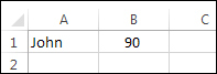
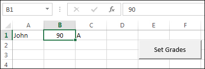
Suppose we had a spreadsheet with a person's name in cell A1 and a score in cell B1. We'd like to examine this score and see if it falls within a certain range. If it's 85 or above, for example, we'd like to award a grade of "A". We want this grade to appear on cell C1. As well as placing a grade in cell C1, we want to change the background colour of the cell. So we want to go from this:

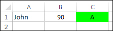
to this:

We want this to happen on the click of a button. How can we do all this with VBA code?

Let's start by breaking the problem down. Here's what will happen:

1. Click inside cell B1
2. Get the value of cell B1
3. Use an If Statement to test the value of cell B1
4. If it's 90 or greater then do the following:
   1. Use an Offset to reference the cell C1
   2. Using the offset, place the text "A" in cell C1
   3. Use the offset to colour the cell C1
   4. As a bonus, we can also centre the text in cell C1

To make a start, go back to your spreadsheet and type a name in cell A1 (the name can be anything you like). Type a score of 90 in cell B1.

Now go back to your coding window. Create a new Sub and call it SetGrades . As the first line of your code, set an integer variable called score :

Dim score As Integer

What we want to do is to place the value from B1 on our spreadsheet inside of this score variable.

To get a value we can from a cell, you can use ActiveCell.Value. This goes on the right of an equal sign:

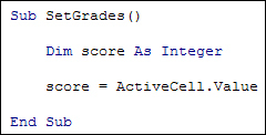
score = ActiveCell.Value

The ActiveCell  is whichever cell is currently selected.

The Value refers to whatever you have typed inside the cell. This Value is then assign to the score variable. Remember: anything you type to the right of an equal sign is what you want to store. The variable on the left of the equal sign is where you are storing it.

But your coding window should now look like this:

Now that we have a score from the spreadsheet, we can test it with an If Statement. We want to check if it's in the range 90 to 100. The If Statement to add to your code is this:

If score >= 90 And score <= 100 Then

End If

You should know what the above does by now. If not, revise the section on conditional and logical operators.

If the score is indeed greater than or equal to 90 and less than or equal to 100 then the first thing we need to do is place an "A" in cell C1.

ActiveCell Referencing

When you use ActiveCell you can point to another cell. You do the pointing with Row and Column numbers. These are typed between round brackets. For example, to point to the currently ActiveCell (the cell you have clicked in to select) the numbers you need to type are 1, 1:

ActiveCell(1, 1).Value

If you want to move one column over from where you are (1, 1) then you add 1 to the Column position:

ActiveCell(1, 2).Value

If you wanted to move one column to the left of where you are, you deduct 1:

ActiveCell(1, 0).Value

To move two columns to the left, you’d need a minus number:

ActiveCell(1, -1).Value

You can move up and down the rows in a similar way – just add or deduct from the first 1 between round brackets.

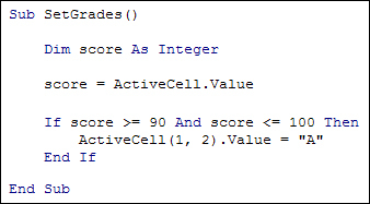
We want to type an "A" in cell C1, which is one column to the right of the ActiveCell. The code to do that is this:

ActiveCell(1, 2).Value = "A"

So we're storing "A" into the Value property of ActiveCell (1,2).

Your coding window should now look like this:

You can test it out at this stage. Go back to your spreadsheet. Add a new button and select SetGrades from the Assign Macro dialogue box. Change the button text to Set Grades . Now click inside your B1 cell, the cell with the score of 90. This will be the ActiveCell referred to in the code. When you click your button, the letter "A" will appear next to it, in cell C1:

There are only two things left to do, now: change the background colour of cell C1 from white to green, and centre the text.

Changing the Background Colour of a Cell

As well as ActiveCell having a Value property, it also has an Interior.Color property, and an Interior.ColorIndex property. You can use either of these to set the background colour of a cell.

If you want to use Interior.Color then after an equal sign, you need to specify an RGB colour:

ActiveCell(1, 2).Interior.Color = RGB(0, 255, 0)

RGB colours use the numbers 0 to 255 to set a Red, a Green, and a Blue component. If you want full Red, you set the R position to 255 and the Green and Blue parts to 0:

RGB(255, 0, 0)

If you want full Green you set its position to 255 and switch the other two positions to 0:

RGB(0, 255, 0)

Likewise, Blue has 255 in its position and 0 in the R and G positions:

RGB(0, 0, 255)

If you want White, you switch all positions to 255:

RGB(255, 255, 255)

If you want Black, you switch all the positions to 0:

RGB(0, 0, 0)

You can have mixture of colours by setting the various positions to any number between 0 and 255:

RGB(255, 255, 0)

RGB(100, 100, 255)

RGB(10, 10, 100)

The Interior.ColorIndex property, on the hand, uses a single number to return a colour:

ActiveCell(1, 2).Interior.ColorIndex = 1

The numbers are built-in constants. This means that the number 1 stands for Black, the Number 2 for White, the number 3 for Red, and so on up to a value of 56.

The problem with using ColorIndex, though, is that the index numbers don't really correspond to a colour – the index number is simply the position of the colour in the Excel colour palette. So the first colour in the palette is index 1, the second colour index 2, the third colour index 3, etc. ColorIndex 4 is a green colour at the moment. But if Microsoft reordered its colour index, the new colour at position 4 might end up being red!

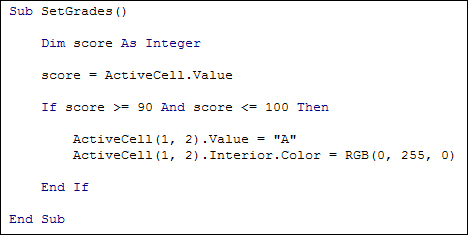
Add the following line to your code:

ActiveCell(1, 2).Interior.Color = RGB(0, 255, 0)

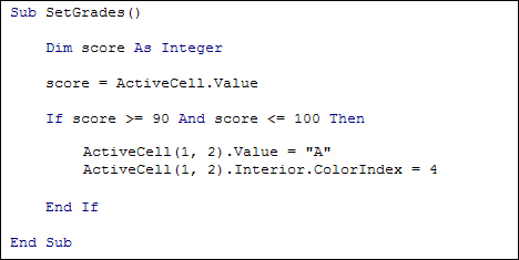
If you like, though, try a ColorIndex instead:

ActiveCell(1, 2).Interior.ColorIndex = 4

Your code will then look like this:

Or like this:

If you want to clear a background colour from a cell you can use the xlColorIndexNone constant:

ActiveCell(1, 2).Interior.ColorIndex = xlColorIndexNone

Cell Content Alignment

You can align data in a spreadsheet cell with the properties HorizontalAlignment and VerticalAlignment . After an equal sign, you then type one of the following constants for HorizontalAlignment:

xlCenter
xlLeft
xlRight

For VerticalAlignment the constants are these:

xlBottom
xlCenter
xlTop

So to align the contents of your cell in the centre, the code would be this:

ActiveCell.HorizontalAlignment = xlCenter

If you wanted to right-align the contents, the code would be this:

ActiveCell.HorizontalAlignment = xlRight

If you only wanted bottom-left for your cell alignment, you only need a vertical alignment of bottom:

ActiveCell.VerticalAlignment = xlBottom

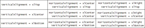
The table below shows all the various alignment position you can have with VBA. The table should be seen as a single cell:

Add one of the alignment options to your own code. Try the following:

ActiveCell. HorizontalAlignment = xlCenter

But the whole of your code should now look like this:

Click your button and try it out. When the code is run, your spreadsheet should look like ours below: