Excel VBA Charts

In this section, you'll learn how to manipulate charts with VBA.

There are two types of chart you can manipulate with VBA code. The first is a chart sheet , and the second is an embedded chart . A chart sheet is a separate sheet in your workbook, with its own tab that you click on at the bottom of Excel. An embedded chart is one that is inserted onto a worksheet. The two types of chart, sheet and embedded, use slightly different code. We'll concentrate on embedded charts. But just to get a flavour of how to create chart sheets with VBA, start a new spreadsheet. Enter some data in cells A1 to B11. Something like the following:

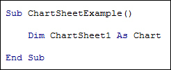
Click Developer > Visual Basic to get at the coding windows. Create a new Sub in Sheet 1. Call it ChartSheetExample . Add the following line:

Dim ChartSheet1 As Chart

Your code should look like this:

So instead of an Integer variable type or a string variable type, we now have a Chart type. The name we've given this Chart variable is ChartSheet1 .

To add a chart sheet, all you need is the call to the Add method. However, we'll set up our ChartSheet1 variable as an object, so that we can access the various chart properties and methods. Add the following line to your code:

Set ChartSheet1 = Charts.Add

Now add a With … End With statement:

With ChartSheet1

End With

The first thing we can do is to add the data for the chart. To do that, you need the SetSourceData method. This method takes a parameter called Source . The Source parameter needs a range of cells to grab data from.

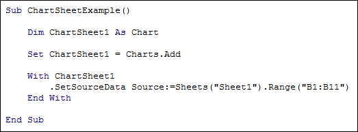
Here's the code to add:

With ChartSheet1

.SetSourceData Source:=Sheets("Sheet1").Range("B1:B11")

End With

After Source:= we have this:

Sheets("Sheet1").Range("B1:B11")

This gets a reference to a Sheet called "Sheet1". The Range of cells we want is cells B1 to B11. Your coding window should now look like this:

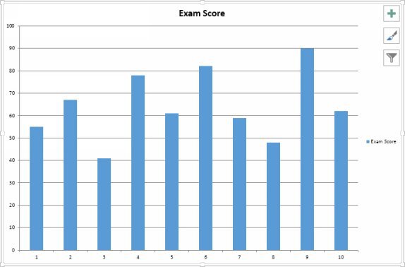
You can run your code at this stage. Press F5 on your keyboard, or click Run > Run Sub/User Form from the menus at the top of the VBA window. You should find that a new Chart sheet opens up in Excel:

Notice that Excel has automatically added a column chart. You can specify what kind of chart you need, however, by using the ChartType property. For the type of column chart Excel has added, you need the enumeration xlColumnClustered :

With ChartSheet1

.SetSourceData

Source:=Sheets("Sheet1").Range("B1:B11")

.ChartType = xlColumnClustered

End With

There are lots of other values (constants) you can add for the ChartType in place of xlColumnClustered. See the Chart Appendix at the end of the book for more details.

The values we added in the A column of the spreadsheet have been used for the X Axis (Category Axis) of the chart sheet, and the scores themselves as the Y Axis (Values Axis). The same text has been used for the chart title and the series legend - "Exam score". You can change all this.

To set a chart title at the top, your first need to switch on the HasTitle property:

.HasTitle = True

You can then set the Text property of the ChartTitle property. Like this:

.ChartTitle.Text = "Chart Sheet Example"

Obviously, between the quotes marks for the Text property, you can add anything you like. This will then be used at the top of the chart.

To set some text below the X and Y Axes, you need the Axes method. After a pair of round brackets, you need two things: a Type and an Axis Group. The Type can be one of the following: xlValue , xlCategory , or xlSeriesAxis (used for 3D charts). The Axis Group can be either xlPrimary or xlSecondary . Add the following to your With Statement:

.Axes(xlCategory, xlPrimary).HasTitle = True

Here, we're switching the HasTitle property on. In between the round brackets of Axes, we've used the xlCategory type then, after a comma, the xlPrimary axis group.

To add some text for the X Axis add this rather long line:

Axes(xlCategory, xlPrimary).AxisTitle.Characters.Text = Range("A1")

Again, we have .Axes(xlCategory, xlPrimary) . This points to the X Axis. After a dot, we then have this:

AxisTitle.Characters.Text

This allows you to set the text. After an = sign, you can either type direct text surrounded by double quotes, or you can specify a cell on your spreadsheet. We've specified the cell A1. Whatever is in cell A1 will then be used as the text for the X Axis.

To set some text for the Y Axis (the Values one), add the following code to your With statement:

.Axes(xlValue, xlPrimary).HasTitle = True
.Axes(xlValue, xlPrimary).AxisTitle.Characters.Text = Range("B1")

This is similar to the code for the X Axis. The difference is that we are now using the xlValue type. We've also set cell B1 to be used as the text.

Your code window should now look like this:

Delete the previous chart and run your code again. The chart that Excel creates should now look like this

We now have a chart with a different chart title. The X Axis has been changed to read "Student Number", and the Y Axis is "Exam Score".

You can delete the chart sheet now, if you like. We'll move on to embedded charts.