Excel Chart Images

Now that we have a chart, we can create an image from it. First, we need a file name and location to save the chart. Add these two lines to your code (the second one is a bit long):

Dim imageName As String

imageName = Application.DefaultFilePath & Application.PathSeparator & "TempChart.gif"

The fileName variable is a string. To get a location to save the file, you can use Application.DefaultFilePath . The default file path is usually the Documents folder in Windows. You can check this location for yourself by adding a message box (one line of code):

MsgBox "The default file path is " & Application.DefaultFilePath

This will tell you where on your computer Excel is going to save the image of the chart. The Application.PathSeparator part just gets you a backslash character ("\"). At the end, you can then type a name for your file. Ours is "TempChart.gif". As well as the GIF format, you can save your images as a JPEG file, or a PNG file. If you want to keep the size of the image file down, though, then use GIF or PNG.

To actually save a file, you need the Export method (one line):

MyChart.Export FileName:= imageName, FilterName:="GIF"

After a space, can have up to three parameters:

FileName - The name of your file
FilterName - An export filter (you get graphics filters when you install Excel/Microsoft Office)
Interactive - Either True or False. (Supposed to display a dialogue box with graphic filters, but doesn't seem to work. You can ignore this parameter.)

We're just using the first two parameters, FileName and FilterName . We're setting FileName to be whatever is in the variable imageName . The FilterName is just whatever format you want to save your image as. If you want to create a JPEG image then change the filter name to JPEG.

When the Export command is run, Excel will save the file for you. If a file of that name already exists then it is overwritten, which is exactly what we want. Nothing else is needed here.

The next step is to delete the chart on the spreadsheet: We need to do this so that we don't have a lot of chart objects embedded in the spreadsheet. The process is quite easy:

ActiveSheet.ChartObjects(1).Delete

All we're doing here is to using the Delete method of the ChartObjects collection. The number between the round brackets is which number chart you want to delete.

Only two more lines to go, now. The first of these is to switch back on ScreenUpdating:

Application.ScreenUpdating = True

The last thing we need to do is to load the saved chart into our Image control:

UserForm1.Image1.Picture = LoadPicture(imageName)

The Image control has a property called Picture . After an equal sign we're then using the LoadPicture method:

LoadPicture(imageName)

In between the round brackets of LoadPicture you type a file path for the image you want to load into your image control. For us, this is contained in the variable called imageName.

And that's it. The whole of your code should look like this:

Test it out. Run your form and select the Arsenal item from the dropdown list. Then click the Load Chart button. You should see this:

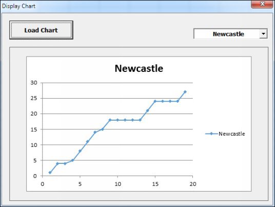
Now select the Newcastle item from the dropdown list. The chart will change to this:

You can quickly see the difference in data as each chart is displayed. And all from a dropdown list on a user form!

In the next part, you’ll tackle a TreeView Project.