Figure 1: Production-Possibilities Frontier
Perhaps the easiest and most concise review of economic concepts is the economics cheer. The cheer is a series of body positions accompanied by the chanting of economic concepts to help you learn the essentials. It might not help you understand the meaning behind the graphs, but it will remind you what they look like. Properly drawn graphs are valuable both as a signal to the grader of intelligent life, and as a springboard to the correct answers that you can often bring to light by visualizing the graphs. The cheer is easy to learn and is performed by making the shapes of different curves with your body. In each case, make the curve so that it looks correct from your own perspective, not that of someone looking at you. Now, follow along (but you might want to do this in private).
“Supply”—Use your left arm to make a line sloping upward to the right.
“Demand”—Use your right arm to make a line sloping downward to the right.
“Equilibrium”—Touch your nose to the point where the demand curve (your right arm) intersects the supply curve (your left arm).
“Elastic”—Represent a perfectly elastic (horizontal) demand curve by placing horizontal arms side by side.
“Inelastic”—Represent a perfectly inelastic (vertical) demand curve by placing arms vertically on either side of your body.
“Substitutes”—Pump one hand up into the air twice, showing that the demand for one item goes up when the price of a substitute goes up.
“Complements”—Pump one hand up and then down, showing that when the price of one item goes up, the demand for a complement goes down.
“Production Possibilities”—Move your left hand back and forth from a twelve o’clock position to a three o’clock position, mapping out the shape of a production possibilities frontier.
“The Floor’s Up High”—Place your arm, with your hand horizontal, above your head to represent an effective price floor (which must be above the equilibrium price).
“The Ceiling’s Down Low”—Place your arm, with your hand horizontal, below your torso to represent an effective price ceiling (which must be below the equilibrium price).
“And That’s the Way the Econ Cheer goes!”—If all onlookers are giggling, you did it right.
Economics is the study of how societies allocate scarce resources among competing ends. Although some think economics is only about business and money, in truth, the field is as broad as the list of scarce resources, and deals with everything from air to concert tickets. Few things have an infinite supply or zero demand, meaning that the need to make choices in response to scarcity—economics—can apply to almost everything and everyone. Even the world’s 1,800-plus billionaires must struggle with constraints in time and resources. That brings us to reason number 493 why economics is great: almost any topic is within its domain. Economists are currently studying war, crime, endangered species, marriage, systems of government, child care, legal rules, death, birth…the sky’s the limit.
Economists view the world in terms of positive economics and normative economics. Positive economics describes the way things are, whereas normative economics addresses the way things should be. For example, “The unemployment rate hit a three-year high” is a positive statement, while “The Fed should lower the federal funds rate” is a normative statement.
Scarcity occurs because our unlimited desire for goods and services exceeds our limited ability to produce them due to constraints on time and resources. The resources used in the production process are sometimes called inputs, or factors of production. They include:
capital—manufactured goods that can be used in the production process, including tools, equipment, buildings, and machinery (this is often referred to as physical capital)
labor—the physical and mental effort of people, including human capital, the knowledge and skill acquired through training and experience
entrepreneurship—the ability to identify opportunities and organize production, and the willingness to accept risk in the pursuit of rewards
natural resources/land—either term can refer to any productive resource existing in nature, including wild plants, mineral deposits, wind, and water
Energy and technology are also important contributors to the production process, but they can be treated as by-products of the four factors of production listed above. Because economists like to work with two-dimensional graphs, the production model is often simplified to include just two inputs: labor and capital.
Consider the factors of production needed for a bagel shop. The shop building, mixers, and ovens are examples of capital. Natural resources, including land and rain, will help provide the wheat for the dough. Labor will form the dough into bagels, place them into the ovens, and sell them. The bagel chef uses her skill and experience—human capital—to make the bagels smooth on the outside and soft on the inside. How did this shop come about? An entrepreneur risked a large amount of money and poured his ideas and organizational talents into the success of the shop. Thus, our bagel shop requires all four factors of production. In contrast, a soda-pop vending machine is an example of a capital-intensive business that requires little beyond canned drinks and the machine itself to produce soft drink sales.
Because economics is the study of the distribution of scarce goods, economists are always looking for ways to analyze human choices. For example, the fact that you are reading this book right now means that you cannot simultaneously be doing a number of other things, like reading the newspaper, swimming, or horseback riding. If the best alternative to reading this book is swimming, then the opportunity cost of reading this book is not being able to go swimming. Opportunity cost is the value of the best alternative sacrificed as compared to what actually takes place. The opportunity cost of going to the prom with Pat may be that you can’t go with Chris. The opportunity cost of going to college may be that you can’t spend the same time working at McDonald’s.
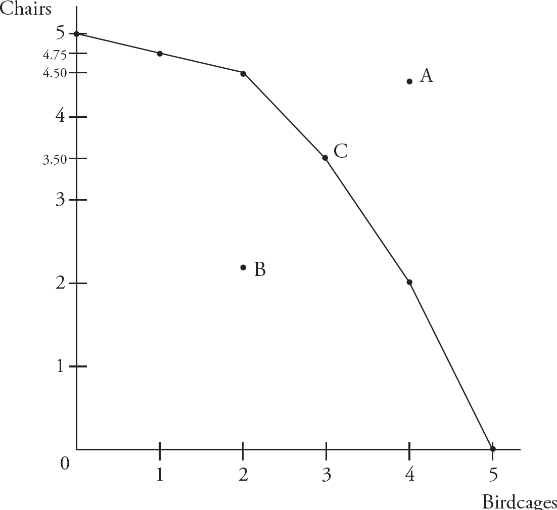
When we use resources to produce one good or service, the opportunity cost is that we cannot produce another good or service. When we make birdcages, we cannot use the same resources to make chairs. The choices an economy faces and the opportunity cost of making one good rather than another can be illustrated with a production-possibilities frontier (PPF). Figure 1 illustrates a production-possibilities frontier for a simplified economy that can use its resources to produce either birdcages or chairs.
Figure 1: Production-Possibilities Frontier
The curve or “frontier” itself represents all of the combinations of the two goods that could be produced using all of the available resources and technology. For example, the economy could produce 5 birdcages and 0 chairs, or 5 chairs and 0 birdcages, or 3 birdcages and 3.5 chairs, and so on.
Birdcage-chair combinations outside the frontier, like point A on the figure, require more resources than the economy has, and are therefore unobtainable. Points inside the frontier are obtainable, but inefficient. Efficiency in this context means that the economy is using all of its resources productively, as is true at every point on the PPF. Producing a birdcage-chair combination that lies inside the PPF, such as point B, results in some resources going to waste. Rather than producing at B, more of both products could be produced by moving to a point such as C on the frontier. Only those points on the frontier itself correspond with the use of all of the available resources.
Resources are often specialized for making one thing rather than another. For example, wood may be ideal for producing chairs, but troublesome as a source of birdcage walls because drilling or carving is necessary to make the birds visible. On the other hand, metal may be simple to weave into a wire birdcage but less than ideal for chairs, because a solid-feeling chair becomes heavy and expensive when made of metal.
When the economy is producing only one good, say chairs, all of the available resources are devoted to that good, including resources that are not especially useful for chair production. Starting from the production of chairs only, the opportunity cost of birdcages—the number of chairs that must be given up to make another birdcage—is initially small because the resources used will be those specialized for making birdcages (metal, plastic, wire-bending machines) and not so useful for making chairs.
Notice that opportunity costs can be read directly off the PPF in Figure 1. Start from the point at which 5 chairs and 0 birdcages are made and stay on the PPF. Making 1 birdcage necessitates a decrease in chair production of 0.25 (from 5 to 4.75). That is, the opportunity cost of the first birdcage is a quarter of a chair. Likewise, the opportunity costs of the second through fifth birdcages are 0.25, 1, 1.5, and 2 chairs respectively. Why does the opportunity cost of making birdcages increase? Because as more birdcages are produced, the resources that must be used to make birdcages are those less and less specialized for birdcage production and more and more specialized for chair production. The economy must therefore give up an increasing number of chairs for each additional birdcage.
The slope of a line between two points is “the rise over the run,” meaning the vertical change divided by the horizontal change between the two points. The absolute value, the value after removing the negative sign, of the slope of the PPF between two points also indicates the average opportunity cost of the horizontal axis good (birdcages) between those two points. This is because the movement from left to right along the horizontal axis, the “run,” indicates an increase in birdcages, while the movement along the vertical axis, “the rise,” indicates the corresponding decrease in the number of chairs. To summarize, the decrease in chairs per increase in birdcages defines both the opportunity cost of birdcages and the slope of the PPF. The slope of the PPF increases in absolute value from left to right, reflecting the increasing opportunity cost of birdcages.
In the special case in which an economy must allocate its resources between two goods that involve no specialization of resources, the PPF will be a straight line. Consider an economy that allocates its resources between radishes and carrots. It may be that the skills, tools, fertilizer, and other resources needed to produce the two goods are virtually identical, and thus the opportunity cost of each good and the PPF slope would not change at different production levels, as in Figure 2.
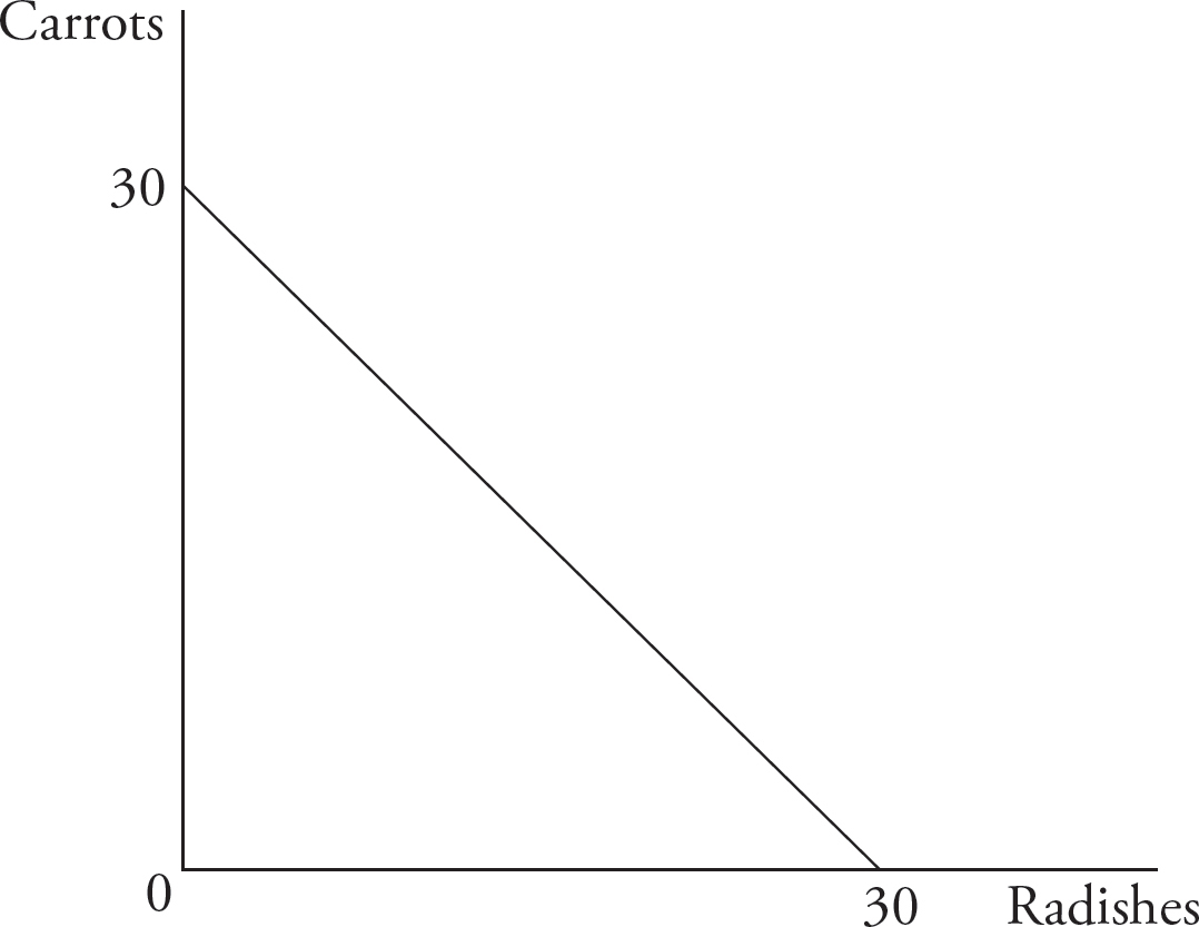
Figure 2
The production-possibilities frontier apparatus is also useful for analyzing production decisions between consumer goods and capital goods. Consumer goods are products that are for sale in any typical retail or consumer market and used directly by consumers. Anything purchased in a supermarket or shopping mall would be a consumer good. Capital goods are things purchased to produce other goods. If a baker decides to invest in an industrial mixer, that mixer would be a capital good. We could use all available resources to produce food, clothing, and other items to be consumed in the present, but that would contribute nothing to our ability to produce goods in the future. Alternatively, we could forgo some current consumption to produce tractors, looms, and other capital goods that add to the ability to produce both capital and consumer goods later on.
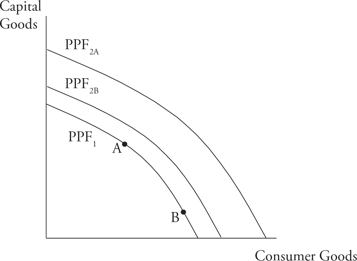
Figure 3
Let PPF1 in Figure 3 represent the production possibilities in Period 1. Point A represents a combination of capital and consumer goods that includes a relatively large investment in capital. The substantial investment in capital comes at the expense of current consumption but allows for considerable growth in future production possibilities as represented by the Period 2 production possibilities frontier labeled PPF2A. Point B represents a production combination that caters to current consumers at the expense of future production. The relatively low level of investment in capital goods results in limited growth in Period 2 as represented by PPF2B. If no capital goods were produced at all, the inability to replace worn-out capital would decrease production possibilities and lead to a Period 2 PPF that fell below the current PPF1. In summary, current investment in capital leads to future growth, so there are important trade-offs between consumption and growth that can be captured with the PPF diagram.
When people have different abilities, having them specialize in what they are relatively good at enhances productivity. Specialization is more efficient than having each person contribute equally to every task. It is better for LeBron James to be a full-time basketball player and Brad Pitt to be a full-time actor than to have them both divide their time equally between the court and the stage. Even if every person were identical, efficiency would be improved by a division of necessary tasks among those carrying out the tasks. This is because such a division of labor permits people to develop expertise in the task(s) that they concentrate on—practice improves performance. If different members of your family specialize in shopping, car repair, cooking, or child care, your family exhibits a division of labor not unlike what occurs in businesses and governmental agencies.
Just as individuals benefit from specialization, so too do larger groups. There are two types of advantages that economists focus on when comparing countries (or other groups of individuals). A country is said to have an absolute advantage in the production of a good when it can produce that good using fewer resources per unit of output than another country. A country is said to have a comparative advantage in the production of a good when it can produce that good at a lower opportunity cost (a smaller loss in terms of the production of another good) than another country. The opportunity for two countries to benefit from specialization and trade rests only on the existence of a comparative advantage in production between the two countries.
Consider Brazil and Mexico and the production of coffee and broccoli. Figure 4 illustrates fictional production-possibilities frontiers for the two countries, simplified to be straight lines.

Figure 4
If we assume that the two countries have identical resources, the PPFs indicate that Brazil has an absolute advantage in both coffee and broccoli, because it can produce more of each good with the same resources. In order to examine comparative advantages, we need to look at the opportunity costs facing each country. When Brazil goes from producing 200 units of broccoli to producing 200 units of coffee, it gives up one unit of broccoli for each unit of coffee, so the opportunity cost of coffee in terms of broccoli is 1. (Because the PPF is a straight line, the opportunity cost is the same for each increment of production.) When Mexico goes from producing 75 units of broccoli to producing 150 units of coffee, it gives up one-half as much broccoli as it increases in coffee, so the opportunity cost of coffee in terms of broccoli is 0.5. Mexico has a comparative advantage in the production of coffee because each unit of coffee costs Mexico 0.5 unit of broccoli, which is less than the opportunity cost of 1 in Brazil. Likewise, Brazil has a comparative advantage in the production of broccoli because each unit of broccoli costs Brazil 1 unit of coffee, which is less than the opportunity cost of 2 units of coffee per unit of broccoli in Mexico.
Because relative production costs differ, these two countries can each benefit from trade. Suppose that in the absence of trade, each country divides its resources equally between the two goods—Brazil produces and consumes 100 units of each, and Mexico produces and consumes 75 units of coffee and 37.5 units of broccoli. A beneficial trade agreement will have each country specialize in the good for which it has a comparative advantage. Mexico should satisfy the two countries’ needs for coffee up to the first 150 units, and Brazil should satisfy the countries’ needs for broccoli up to the first 200 units. As an example of a mutually beneficial trade situation, Mexico could produce 150 units of coffee, and Brazil could produce 150 units of broccoli and 50 units of coffee. Mexico could then trade 60 units of coffee for 40 units of broccoli—representing an exchange price of 1.5 units of coffee per unit of broccoli. Because Brazil and Mexico have opportunity costs for broccoli of 1 and 2 respectively, any exchange price for broccoli between 1 and 2 will give Brazil more than its production cost and allow Mexico to purchase at less than its private production cost. After the trade, Brazil can consume 110 units of broccoli and 110 units of coffee, while Mexico can consume 40 units of broccoli and 90 units of coffee. In the end, each country can enjoy more of each good than if it did not trade because, remember, we supposed that in the absence of trade Brazil produced and consumed 100 units of each, and Mexico produced and consumed 75 units of coffee and 37.5 units of broccoli. In other words, with trade, each country enjoys a consumption possibilities frontier that exceeds its production possibilities frontier. The slope of the consumption possibilities frontier is determined by the terms of trade.
The demand curve displays the relationship between price and the quantity demanded of a good within a given period. For example, Figure 5 indicates that Davon would purchase 6 avocados at a price of 25 cents each and 3 avocados at a price of 95 cents each.

Figure 5: The Demand Curve
An individual’s demand curve for a good reflects the additional benefit or “marginal utility” (measured in dollars) received from each incremental unit of the good. Davon values the first avocado at $1.50, the second at $1.20, the third at $0.95, and so on. A line through the points on this graph makes a demand curve. The same information is represented in Table 1, which is known as a demand schedule.
|
Price (dollars per avocado) |
Quantity of avocados demanded |
|
1.50 |
1 |
|
1.20 |
2 |
|
0.95 |
3 |
|
0.63 |
4 |
|
0.50 |
5 |
|
0.25 |
6 |
Table 1
Notice that Davon receives less and less additional benefit—his marginal utility decreases—as he gets more and more avocados. That first avocado will go toward his greatest need, perhaps extreme hunger. However, as he consumes more avocados, he becomes less hungry, and his avocados are used to satisfy less and less important needs (e.g., feeding the cat, batting practice). The decreasing satisfaction gained from additional units of a good consumed in a given period is called the law of diminishing marginal utility.
The law of diminishing marginal utility corresponds with the law of demand, which states that as the price of a good rises, the quantity of that good demanded by consumers falls. Similarly, as the price of a good falls, the quantity demanded of that good rises. Davon would buy three avocados at a price of 75 cents because each of the first three is worth more than 75 cents to him, but the fourth and subsequent units are worth less than 75 cents to him, so he wouldn’t buy them. If the price fell to 35 cents, the quantity he demanded would increase, because then the fourth and fifth avocados (in addition to the first, second, and third as before) would be worth more to him than the price. This explains the inverse relationship between prices and the quantity demanded suggested by the law of demand.
The market demand curve is found by simply adding up the demands of all the individual demanders in the market. For simplicity, assume that Davon and Mary are the only two purchasers of avocados (perhaps they share a tropical island). Figure 6 exhibits the individual demand curves for Davon and Mary and the associated market demand curve.
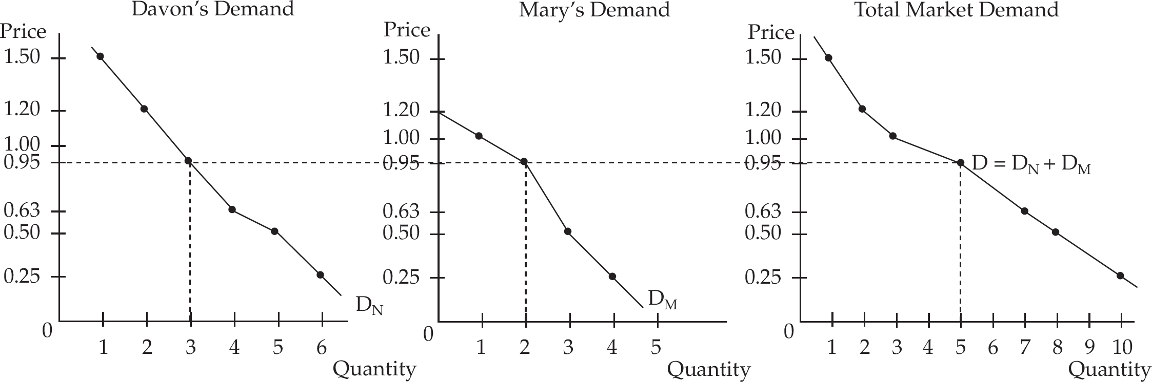
Figure 6
At each price, the market demand curve combines the demand curves of the two consumers. At $1.50 Davon purchases one and Mary purchases zero so the market demand is one. At $0.95, Davon purchases three and Mary purchases two, so the market demand is five, and so on.
The standard supply and demand model is built upon the assumption of a perfectly competitive market, meaning that many small firms sell the same product and can enter or leave the market without cost.
The supply curve (Figure 7) for a perfectly competitive firm and the corresponding supply schedule (Table 2) show the relationship between price and quantity supplied by that firm within a given period.
The law of supply says that as the price increases, the quantity of a good supplied in a given period will increase, other things being equal. Think about how many avocados you would be willing to supply at different prices. At a price of $0.25 you probably wouldn’t be very enthused about the prospects, but perhaps you would be willing to give up some of your least valuable time—the time you spend watching The Simpsons reruns—to grow 100 avocados as a hobby. With such a low return, you might not want to give up your second-least-favorite pastime of picking on your sibling. However, if the price rose to $0.50 per avocado, forget picking on your sibling; you might be willing to spend more time and invest more money into growing 200 avocados.
Although efficiencies may come about in the beginning, eventually the additional cost of producing another unit—the marginal cost—will increase for several reasons. The opportunity cost of your time will increase as you have to give up more and more valuable alternatives in order to grow more avocados. You will start by hiring the best and cheapest inputs (avocado pickers, tractors, land) and then resort to inferior inputs as necessary. You might get less and less out of each additional unit of an input as opportunities for efficient specialization are exploited and you run into redundancy and congestion (for more on this, see the Marginal Product and Diminishing Returns section in Chapter 7). For all of these reasons, higher prices are needed to induce more avocado production, and the supply curve and schedule might look something like Figure 7 and Table 2, respectively.
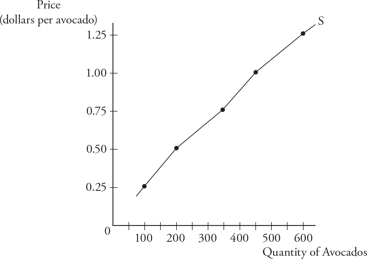
Figure 7: The Supply Curve
|
Price (dollars per avocado) |
Quantity of avocados supplied |
|
1.25 |
600 |
|
1.00 |
450 |
|
0.75 |
350 |
|
0.50 |
200 |
|
0.25 |
100 |
Table 2
The market supply curve indicates the total quantities of a good that suppliers are willing and able to provide at various prices during a given period of time. It is the horizontal summation of all of the firm supply curves. Figure 8 illustrates how the supply curves of two firms are added to find the market supply.
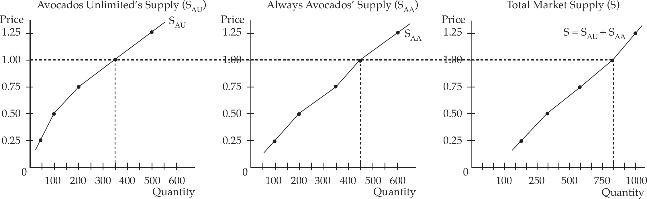
Figure 8
For example, if Avocados Unlimited is willing to produce 350 avocados for $1 each, and Always Avocados is willing to produce 450 at $1 each, and these are the only two producers in the market, then the market supply is 350 + 450 = 800 at a price of $1. The market supply curve reflects the marginal cost (MC) of producing various quantities of a good and the size and number of firms in the market (see Chapter 7 for a discussion of when a firm will shut down and supply zero).
The demand curve and the supply curve for a particular good live on the same graph with price on the vertical axis and quantity on the horizontal axis. Because the consumer’s marginal utility (additional benefit) from the first few units of a good is often relatively high and the supplier’s marginal (additional) cost of producing the first few units is often relatively low, the demand curve begins above the supply curve as in Figure 9.

Figure 9
The point of intersection between the two curves is called the equilibrium point. It is only at the equilibrium price of $1,500 that the quantity of computers demanded equals the quantity supplied (900). For that reason, the equilibrium price is also called the market clearing price. If the price were above $1,500—say, $3,000—the 1,000 computers supplied would exceed the 700 demanded. The resulting surplus of 300 computers would lead sellers to lower their prices until equilibrium is reached. Likewise, if the price were below $1,500, say $500, a shortage of 600 computers would exist because the 1,200 demanded would exceed the 600 supplied. With lines out their doors for computers, the computer sellers would raise their prices until equilibrium was reached. Economic theory predicts that in the long run the market price and quantity will equal the equilibrium price and quantity.
economics
scarcity
positive economics
normative economics
resources
inputs
factors of production
labor
human capital
physical capital
entrepreneurship
natural resources
land
opportunity cost
trade-offs
production-possibilities frontier
efficiency
slope
absolute value
demand
demand curve
demand schedule
law of demand
law of diminishing marginal utility
supply
supply curve
supply schedule
market supply curve
law of supply
marginal cost
equilibrium
market clearing price
surplus
shortage
specialization
productivity
division of labor
absolute advantage
comparative advantage
consumption-possibilities frontier
terms of trade
See Chapter 9 for answers and explanations.
1. A demand curve slopes downward for an individual as the result of
(A) diminishing marginal utility
(B) diminishing marginal returns
(C) the Fisher effect
(D) diminishing returns to scale
(E) increasing marginal cost
2. The supply curve for lawn-mowing services is likely to slope upward because of
(A) decreasing marginal costs
(B) increasing opportunity cost of time
(C) diminishing marginal utility
(D) increasing returns to scale
(E) economies of scope
3. If both supply and demand increase, the result is
(A) a definite increase in price and an indeterminate change in quantity
(B) a definite increase in quantity and an indeterminate change in price
(C) a definite decrease in quantity and an indeterminate change in price
(D) a definite decrease in price and a definite increase in quantity
(E) a definite increase in price and a definite increase in quantity
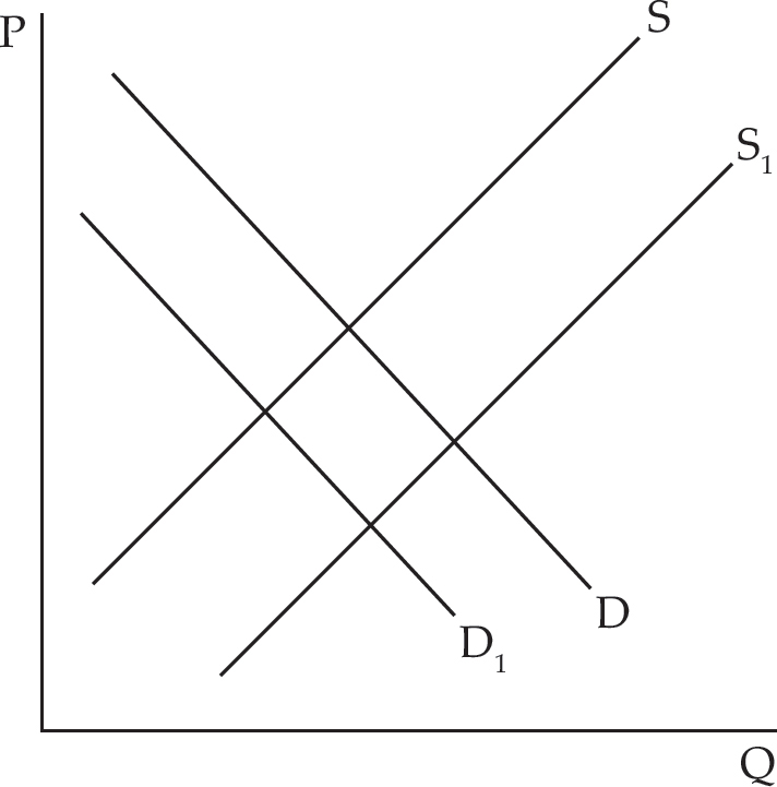
4. For the market supply and demand graph above, when the demand curve shifts from D to D1 and the supply curve shifts from S to S1, then
(A) the equilibrium price falls and the equilibrium quantity is undetermined
(B) the equilibrium price falls and the equilibrium quantity is unchanged
(C) the equilibrium price is unchanged and the equilibrium quantity rises
(D) the equilibrium price is undetermined and the equilibrium quantity falls
(E) None of the above
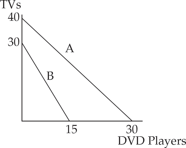
5. The above diagram represents the production possibilities of Country A and Country B, with the use of the same resources. Which of the following would be true for both Country A and Country B?
(A) Countries A and B cannot benefit from trade with each other.
(B) Country A has a comparative advantage in TVs and Country B has a comparative advantage in DVD players.
(C) Country A has a comparative advantage in DVD players and Country B has a comparative advantage in TVs.
(D) Country A has an opportunity cost of 1 DVD players when they produce 1 TV.
(E) Country B has an opportunity cost of  TV when they produce one DVD player.
6. Which of the following would NOT be considered a factor of production for a car company?
(A) the cost of the car designer’s studio
(B) the car designer’s time
(C) the car designer’s creativity
(D) the car designer’s preference for designing homes instead of cars.
(E) the steel and rubber used in car production.
Positive economics describes the way things are; normative economics describes the way things should be.
Economics is the study of how to allocate scarce resources among competing ends.
The resources used in the production process are called inputs, or factors of production. They include the following factors:
capital
labor (human capital)
entrepreneurship
natural resources/land
Opportunity cost is the value of the best alternative sacrificed as compared to what actually takes place.
A production-possibilities frontier is a curve that represents all of the combinations of the two goods that could be produced using all of the available resources and technology.
Efficiency in this context means that the economy is using all of its resources productively, as is true at every point on the PPF.
The division of labor permits people to develop expertise in the task(s) that they concentrate on.
A country is said to have an absolute advantage in the production of a good when it can produce that good using fewer resources per unit of output than another country.
A country is said to have a comparative advantage in the production of a good when it can produce that good at a lower opportunity cost than another country.
The demand curve illustrates the law of demand that describes the inverse relationship between price and the quantity demanded of a good within a given period.
The law of diminishing marginal utility states that consumers will experience decreasing satisfaction from additional units of a good consumed.
The supply curve illustrates the law of supply that says that as the price increases, the quantity of a good supplied in a given period will increase, other things being equal.
The marginal cost is the additional cost a supplier faces when producing one more unit of a good.
The market supply curve indicates the total quantities of a good that suppliers are willing and able to provide at various prices during a given period of time.
The equilibrium point is the price at which the quantity demanded of a good equals the quantity supplied of a good.
A surplus occurs when too many of a good are provided; a shortage occurs when too few of a good are provided.