Figure 1
Remember that the law of demand says that as the price of a good decreases, the quantity of demanded will also decrease, all other things being held equal. In this chapter, you will study how and why the law of demand holds true. You will also study how and why demand changes.
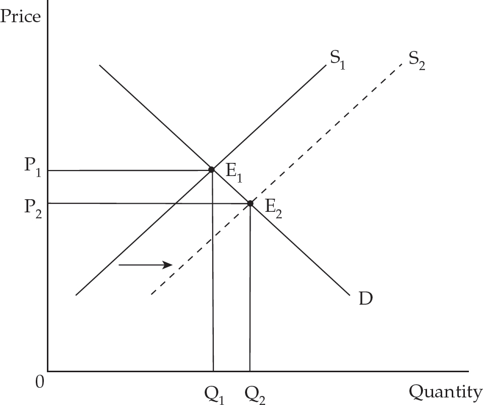
It is important to distinguish between a change in the quantity demanded and a change in demand. A movement of the equilibrium along a stationary demand curve represents a change in the quantity demanded.
Figure 1
For example, when the supply increases from S1 to S2 in Figure 1, the equilibrium moves from E1 to E2, and the equilibrium price moves from P1 to P2. This results in a change in the quantity demanded from Q1 to Q2. Because the demand curve shows the relationship between quantity demanded and price, changes in price simply bring us to different points on the same demand curve, thereby causing changes in the quantity demanded. In contrast, a shift in the demand curve represents a change in demand. Keep in mind that the demand curve maps out the value of each additional unit of a good to consumers. A shift in demand would result from any change that affects the value of that good to consumers or the number of consumers in the market.
Anything other than a lower price that induces increased consumption of a good causes a shift to the right of the demand curve as in Figure 2.
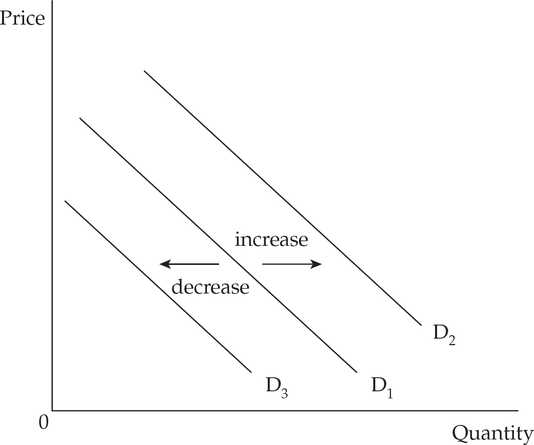
Figure 2: Shifts in Demand
Specifically, an increase (shift to the right) in demand can result from the following:
A positive change in tastes or preferences. Such a change could result from a successful advertising campaign or a research report finding the good to have positive effects on health.
An increase in the price of substitute goods. For example, if the price of Pepsi goes up, the demand for Coke will increase.
A decrease in the price of complements. For example, if the price of gasoline goes down, the demand for large cars will increase.
An increase in income for normal goods. (By definition, a normal good is one that the consumer buys more of when income increases.) For example, a higher income might lead to a higher demand for steak.
A decrease in income for inferior goods. (By definition, an inferior good is one that the consumer buys more of when income decreases.) For example, a lower income might lead to a higher demand for hot dogs if people start substituting them for steak.
An increase in the number of buyers. With more buyers, more individual demand curves are added to find the market demand curve.
Expectations of higher future income. If you pass your board exam and realize you’re going to make big money, you will probably start spending more now. This is called consumption smoothing.
Expectations of higher future prices. This is a good reason to buy more now rather than later.
Expectations of future shortages. For example, when a severe storm is predicted, people often stock up on canned goods and bottled water beforehand.
Lower taxes or higher subsidies. Either of these changes will make more money available for consumption.
Regulations that promote use. For example, the adoption of regulations that require fire alarms in every room of the house would increase the demand for fire alarms.
Of course, the opposite of each of the above changes will cause the demand curve to decrease (shift to the left). Remember, changes in the price of a good do not change the demand for that good. They change only the quantity demanded. This is because changes in the price of a good do not change the value of that good to us. They change only the quantity of the good that we can buy before the value of the good falls below the price.
You can remember the primary reasons for a shift in demand with the acronym TRIBE.
T – Tastes and preferences of consumers
R – the prices of Related goods (substitutes and complements)
I – the Income of buyers
B – the number of Buyers
E – Expectations for the future
Let’s explore how shifts in both supply and demand affect each other. It can be confusing to sort out in one’s head but easy to determine by simply drawing the graph.
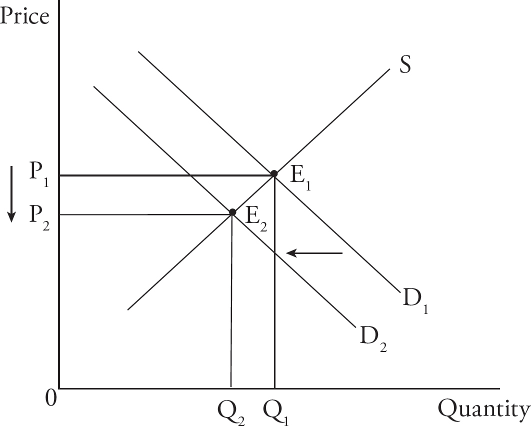
Figure 3
If demand decreases (for example, as the result of a decrease in income), a comparison of the old and new equilibrium price and quantity in a quick sketch like Figure 3 will immediately indicate that both price and quantity decrease.
It is a common mistake on AP exams to shift both supply and demand when only one of the two should be shifted. Think carefully about whether the influence described in an exam question will affect production costs and therefore the supply curve, or consumers’ willingness and ability to pay and therefore the demand curve.
It is always possible that two influences will occur at once. Suppose there is a massive beetle infestation in the farm belt and at the same time a study finds that carrots prevent heart disease. The beetles will increase the cost of producing carrots and thus decrease their supply. The study will increase consumers’ willingness to pay for carrots and thus increase the demand. Figure 4 illustrates the new equilibrium.

Figure 4
Whenever both supply and demand shift at the same time, the effect on equilibrium price OR quantity will be certain, and the effect on the other will depend on the relative size of the shifts in supply and demand. In Figure 4 it is clear that the equilibrium price increases, because both a decrease in supply and an increase in demand result in a higher price. However, because a decrease in supply decreases the equilibrium quantity and an increase in demand increases the equilibrium quantity, the net effect on quantity depends on the relative sizes of the shifts. As it is drawn here, the supply shift dominates the demand shift and there is a net decrease in quantity. Don’t let supply and demand-shifting questions intimidate you; simply draw the graph and describe the evident outcomes. It may help to label clearly the original equilibrium and the new equilibrium so that you don’t get confused about the four points of intersection while you are interpreting the graph. When both supply and demand shift and you do not know the relative size of the shifts, it is appropriate to state that the change in the variable (price or quantity) that is pulled in both directions is “indeterminant” (cannot be determined).
A tip on shifting curves: It can be confusing that a decrease in supply shifts the supply curve up, while a decrease in demand shifts the demand curve down. To clear things up, remember that for both curves, Left is Less and Right is Rising!
Remember that utility is a measure of individuals’ satisfaction. Marginal utility (MU) is the additional utility gained from consuming one more unit of a good and is often quantified in terms of the amount of money an individual would be willing to spend on that good. The principle of diminishing marginal utility suggests that as one consumes more and more of a good, the additional satisfaction gained from subsequent units (MU) decreases.
Suppose the dollar value of Austin’s marginal utility from cheese slices is as indicated in Figure 5 and Table 1.
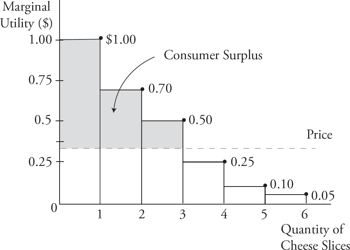
Figure 5
|
Quantity of Cheese Slices |
Marginal Utility (in dollars) |
Total Utility (in dollars) |
|
1 |
1.00 |
1.00 |
|
2 |
0.70 |
1.70 |
|
3 |
0.50 |
2.20 |
|
4 |
0.25 |
2.45 |
|
5 |
0.10 |
2.55 |
|
6 |
0.05 |
2.60 |
Table 1
The first slice is worth $1.00 to him, the second is worth 70 cents, and so forth. He will choose to consume until one more slice would be worth less to him than the price. If the price were $0.35, he would consume the first three, which are worth $1.00, $0.70, and $0.50 to him. He would not pay $0.35 for the fourth slice, which is worth only $0.25 to him. The points drawn on this graph outline Austin’s demand curve, and tell us everything we need to know to calculate his total utility and consumer surplus (explained below).
Total utility is found by adding the marginal utility values gained from each of the units consumed. Because Austin consumes three slices of cheese, his total utility is $1.00 + $0.70 + $0.50 = $2.20. More generally, the relationship between marginal utility and total utility is as illustrated in Figure 6 on the next page. As more and more of a typical good is consumed, the total utility received from that good increases at a decreasing rate, reaches a peak, and then decreases at an increasing rate. This is because marginal utility—the contribution to total utility from the last unit consumed—diminishes as more of the good is consumed. Total utility reaches a maximum at the quantity for which marginal utility is zero, after which point each additional unit provides a negative marginal utility and therefore detracts from total utility.
Take note of the graphical relationship between the curves representing total and marginal utility: the marginal utility at any particular quantity is the slope of the total utility curve at that quantity. Thus, when marginal utility is positive, total utility is rising with a positive slope. When marginal utility is zero, total utility is at a peak with a zero slope. When marginal utility is negative, total utility is declining with a negative slope.

Figure 6: Total Utility and Marginal Utility
Consumer surplus is the value a buyer receives from the purchase of a good in excess of what is paid for it. With a price of $0.35 for the first, second, and third slices, Austin receives consumer surpluses of $1.00 – $0.35 = $0.65, $0.70 – $0.35 = $0.35, and $0.50 – $0.35 = $0.15, respectively. To be more general, consumer surplus is the area below the demand curve and above the price line up to the quantity that is consumed. Producer surplus is the difference between the price a seller receives for a good and the minimum price for which she would be willing to supply a quantity of the good. Producer surplus is thus the area below the price line and above the supply curve. Figure 7 illustrates consumer surplus and producer surplus in a general case.
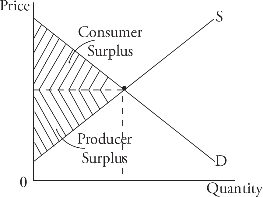
Figure 7: Consumer and Producer Surplus
The distinction between total and marginal utility helps to sort out a paradox that dates back to Plato. It may seem strange that we pay very little money for some goods, such as water, which are essential to life, while we pay much more money for some goods that are inessential, such as diamonds. Although the value of water is very high, this value is reflected in the total utility gained from it, not in the marginal utility. Because water is plentiful, we consume it until the marginal utility is very small. In contrast, diamonds are scarce, so although the initial units are worth less to us than the life-sustaining first units of water, supply restricts our consumption of diamonds to a point where the marginal utility is still very high.
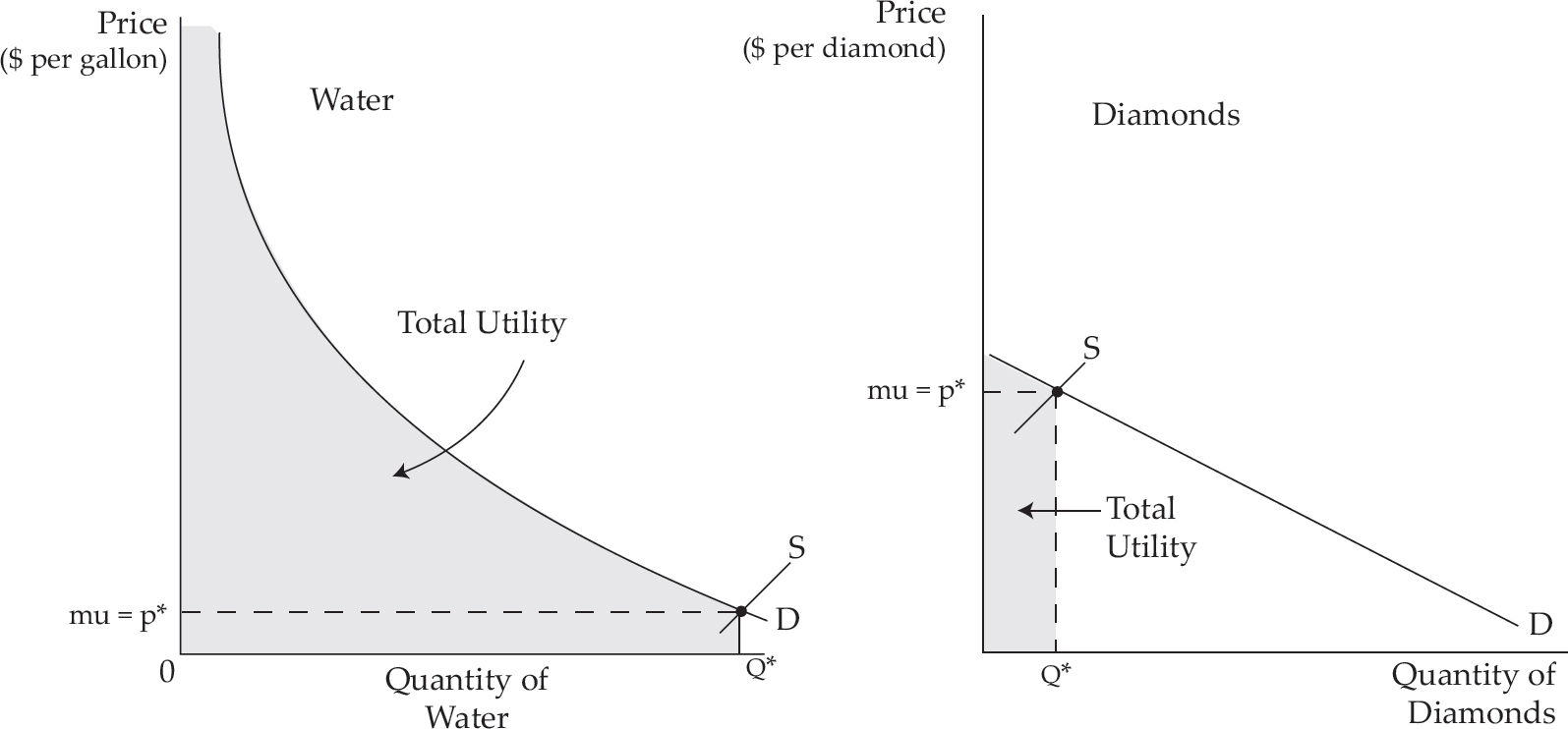
Figure 8: The Water–Diamond Paradox
In Figure 8, notice that the total utility from water is much larger than that for diamonds, but the marginal utility is much smaller for water than for diamonds. Thankfully, price corresponds with the marginal utility rather than the total utility.
Elasticity indicates how responsive consumer behavior is to changes in the product or service they want. In this section we will discuss changes in the product or service they want.
Suppliers often consider how changes in the price of a good or service will affect demand for that good or service. If the price of gum increased by 50 percent from 4 cents to 6 cents, by what percent would the quantity demanded decrease? How many fewer people would buy a ticket for a vacation cruise if the cost increased by 50 percent from $1,000 to $1,500? The price elasticity of demand indicates how responsive the quantity demanded of a good is to price changes. In other words, when economists think about the price elasticity of demand, they’re thinking about how sensitive consumer behavior is to changes in the price of a good. Generally speaking, when consumer behavior is affected by price, the good is elastic; When consumer behavior is unaffected by changes in price, the good is inelastic. The elasticity (responsiveness to price changes) of a good’s demand tends to relate to the following factors:
The proportion of income spent on the good. If a good represents a high proportion of a consumer’s income, the demand for the good will likely be elastic. Consider the gum and cruise price-change scenarios mentioned above. The quantity of cruises purchased will probably be more affected by a 50 percent price increase than the quantity of gum, because an extra 2 cents is not a big deal, but an extra $500 is more likely to be prohibitive. In other words, consumers are more sensitive to a particular percent change in price at higher price levels.
The availability of close substitutes. If there are many substitutes available, the demand for the good will likely be elastic. For example, if there are 10 brands of bicycles available and the price of one of them increases, the quantity of that brand demanded is likely to fall a lot. On the other hand, the demand for bicycles as a whole is less elastic than the demand for a particular brand because the substitutes for bikes in general—cars, skateboards, walking—are not as close.
The importance of the good. The less essential a good is, the more likely consumers are to forego the good when it becomes more expensive. If a good is very important to the consumer, the consumer will continue to purchase it even if the price changes, and demand for that good will be inelastic.
The ability to delay the purchase of the good. When time is short, it is more difficult to change purchasing patterns in response to price changes; therefore, when less time is available, demand for a given good is less elastic. The more time consumers have to adapt, the more they are able to find substitutes or learn to do without goods whose prices have increased.
When thinking about elasticity, economists divide goods into three groups: elastic, unit elastic, and inelastic. If the percentage change in quantity demanded exceeds the percentage change in price for a particular good—meaning, for example, that a 50 percent price increase results in more than a 50 percent decrease in quantity demanded—the demand for that good is on the more price-sensitive side and is labeled elastic. Goods with an elastic demand are categorized as luxuries. If the percentage change in quantity demanded equals the percentage change in price, demand for the good is labeled unit elastic. If the percentage change in quantity demanded is less than the percentage change in price, the demand is labeled inelastic and the good is categorized as a necessity.
Allowing Δ to represent change and Qd to represent the quantity demanded, the formula for price elasticity is the percentage change in quantity demanded divided by the percentage change in price:
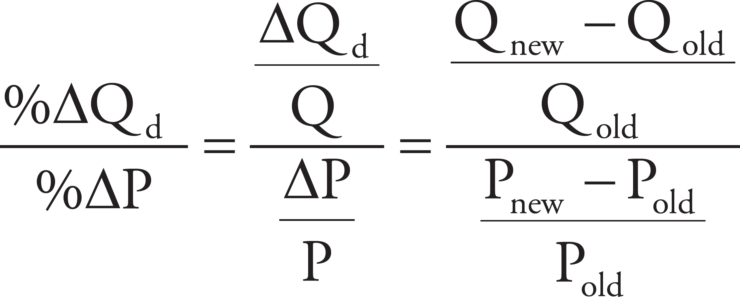
The above formula uses the initial price and quantity as the basis for calculating the percentage change. Although this is the simplest way to do it, the following formula is more precise, especially when the changes in price or quantity are large:
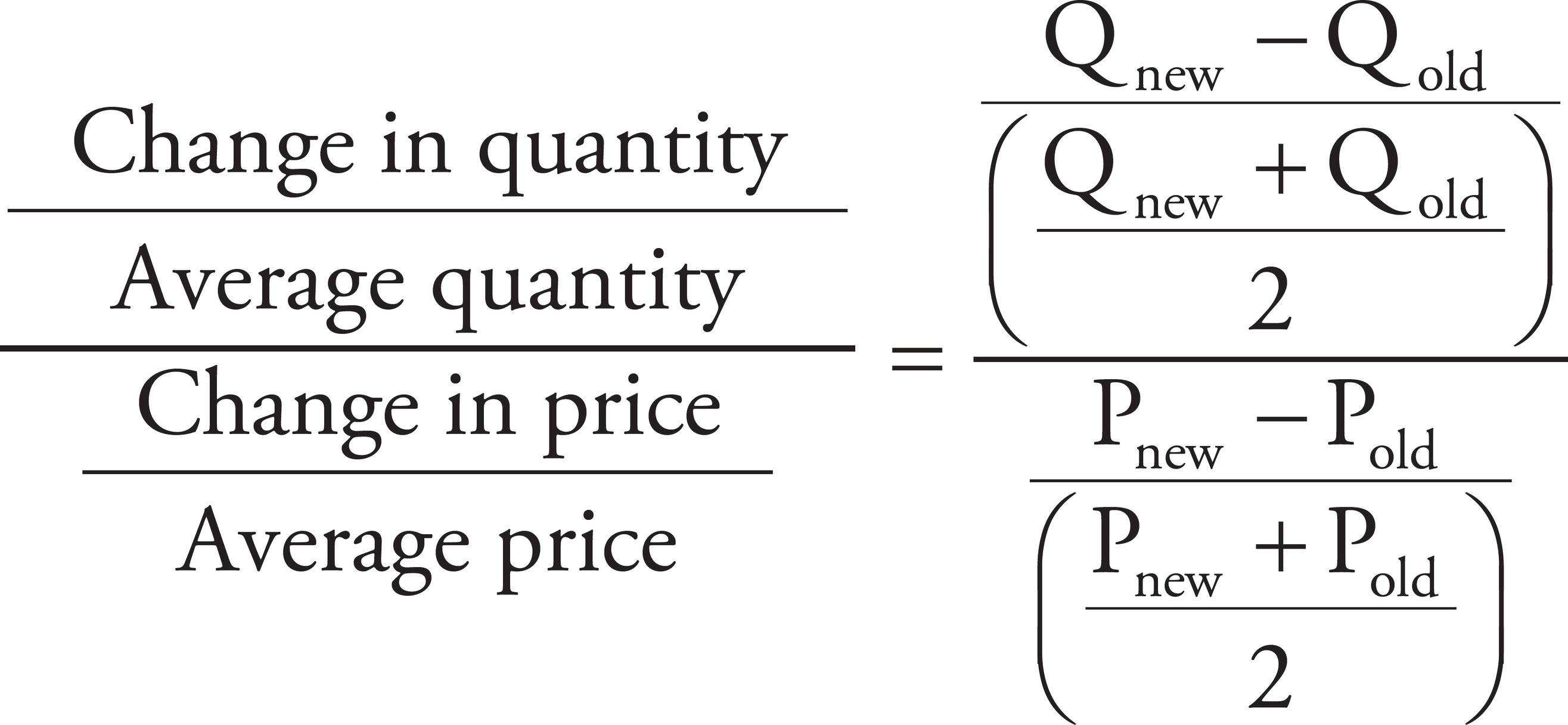
This is more precise because a percent increase in price or quantity is different from a percent decrease in price or quantity over the same range. Here’s an example: a percent increase from $4 to $5 = 25 percent, whereas a percent decrease from $5 to $4 = 20 percent.
Conveniently, the second formula produces the same elasticity measure between two points on a demand curve, regardless of which point you consider the “old” point and which you consider the “new” point. Finding the elasticity measure is simply a matter of plugging in the new and old price and quantity.
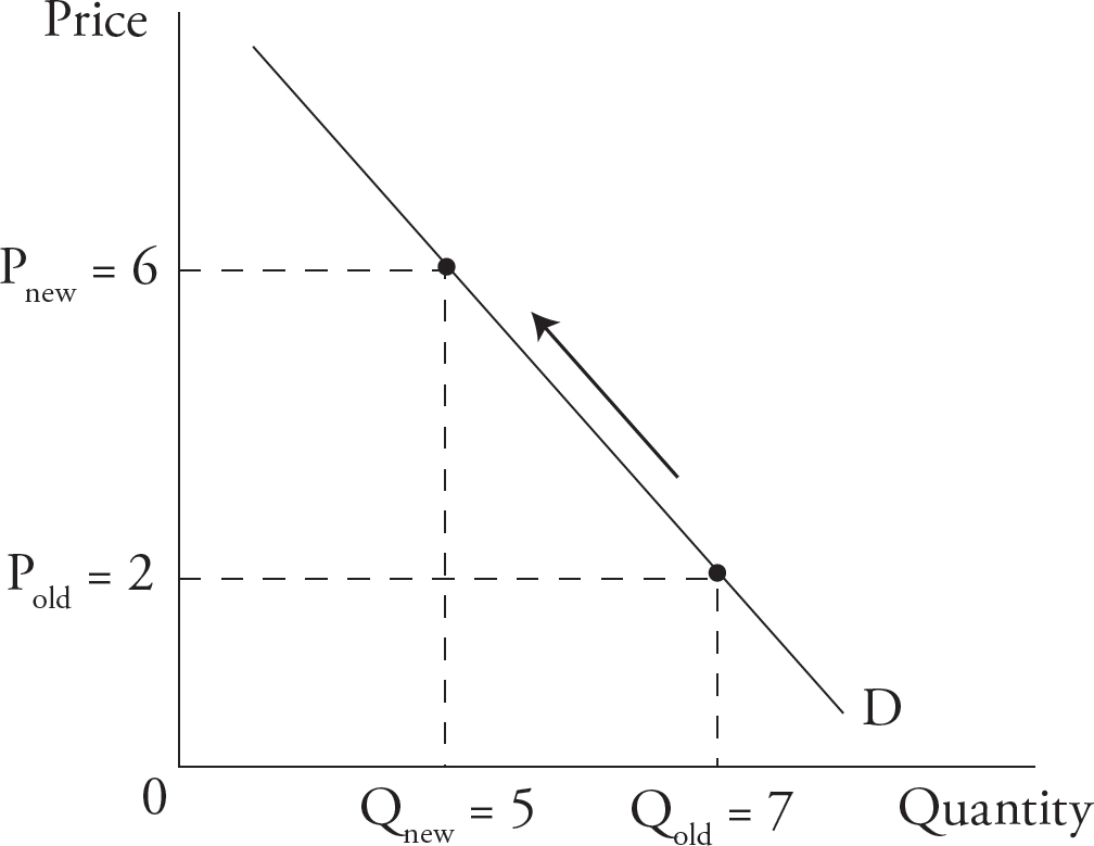
Figure 9
For example, the price elasticity of demand in the range shown in Figure 9 is
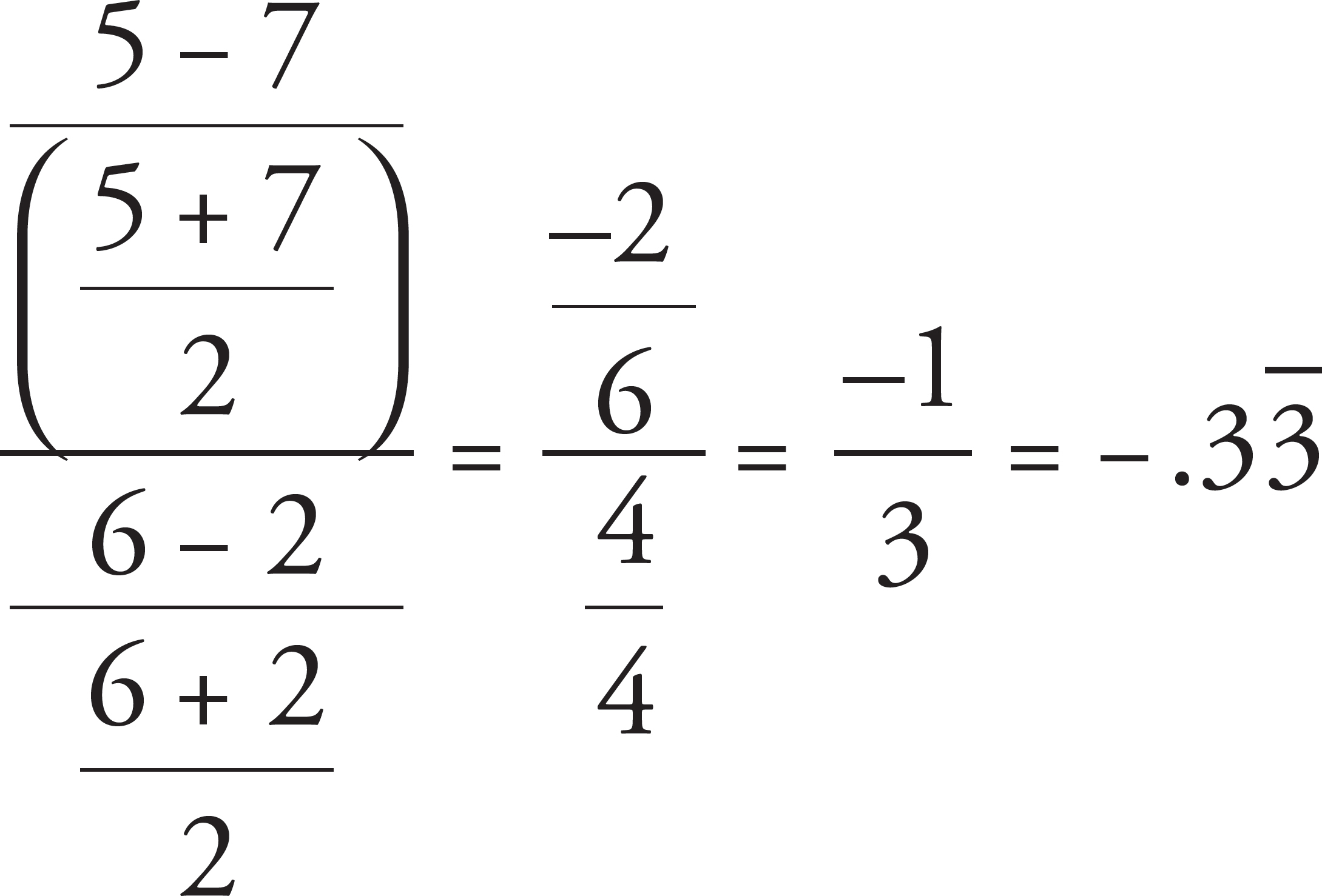
Because the elasticity quotient is less than one, the demand is inelastic. In this equation, 1 is the critical number in determining elasticity. If the quotient is less than 1, as is the case here, then the denominator (%ΔP) is greater than the numerator (%ΔQd), and the good is therefore inelastic. If the numerator and the denominator are equal, the result is 1, and the good is unit elastic. If the result is greater than 1, then the numerator is greater than the denominator, and the good is elastic.
Keep in mind that the results for the equation to determine elasticity will always be negative given the law of demand. As the law of demand says, an increase in price should result in a decrease in the quantity demanded, and a decrease in price should result in an increase in the quantity demanded. Because price and quantity demanded are always going in opposite directions, either the top or the bottom of the elasticity formula will always be negative and the other half will be positive. Either way, the elasticity of demand will come out negative. This being the case, it is conventional to drop the negative sign (take the absolute value) and refer to price elasticities in positive terms. The above elasticity would thus be  .
.

Figure 10
The elasticity of demand relates to the slope of the demand curve, but it does not equal the slope of the demand curve. Note the difference:
slope 
elasticity 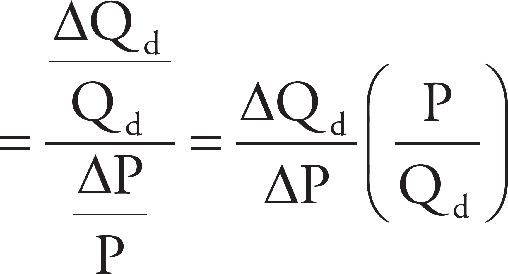
Looking at the last part of each equation, you can see that elasticity is the inverse of the slope multiplied by price over quantity. The relationship between slope and elasticity is such that for a given P and Q, a steeper demand curve (one with a greater slope) is less elastic than a flatter demand curve (one with a smaller slope). A vertical demand curve as in Figure 11 is called perfectly inelastic because price has no influence on the quantity demanded and the elasticity value is 0.

Figure 11: Perfectly Inelastic Demand
This approximates the demand for a lifesaving operation, insulin for a diabetic person, or a drug to which the user is addicted.
A horizontal demand curve, as in Figure 12, is called perfectly elastic because any increase in price will result in a quantity demanded of zero and the elasticity value is infinite.

Figure 12: Perfectly Elastic Demand
This approximates the demand curve facing a corn farmer. As one of thousands of sellers of an identical product, she can sell all she wants at the price set by the market, but if she raises her price even one cent, no one will buy from her, because there are thousands of others selling the same product for the lower price. Because of price regulations, she is unable to lower her price.
A straight line demand curve, as in Figure 13, will have different elasticities at different points along the curve.
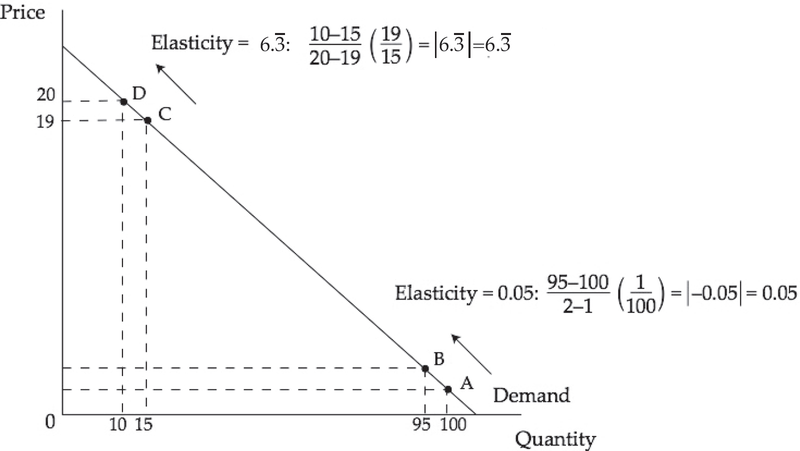
Figure 13
Note that the elasticity moving from point A to point B is 0.05 while the elasticity moving from point C to point D is 6.3 even though the price and quantity changes are of the same size. More generally, the elasticity along a straight line demand curve will go from infinity to 0 moving left to right as illustrated in Figure 14.
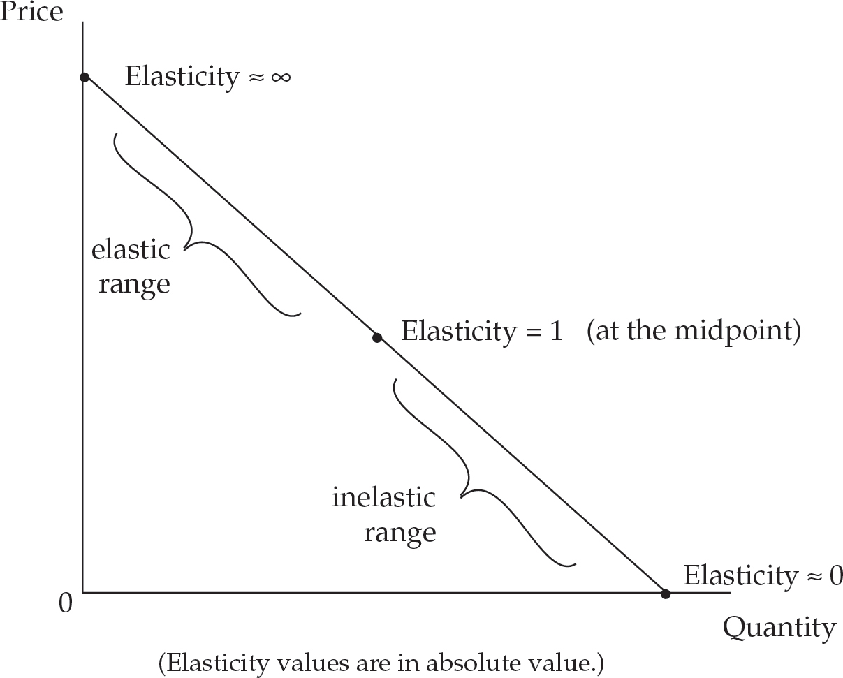
Figure 14
Why should a business care about the elasticity of demand? One reason is that the elasticity determines what happens to revenue when price changes. Note that total revenue (TR) equals price times quantity, which can be graphically related to the area of a rectangle that has a length equal to the price and a width equal to the quantity (length × width equals the area of a rectangle). Figure 15 illustrates three demand curves: one relatively inelastic, one unit elastic, and one relatively elastic.
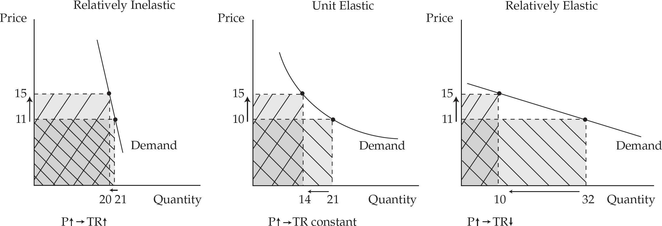
Figure 15
The price in each case has risen by the same amount. Nonetheless, it is clear that revenue (the area of the rectangle) has increased in the inelastic case, stayed the same in the unit elastic case, and decreased in the elastic case. Thus, businesses should remember this rule: when facing an inelastic demand, the best way to bring in more revenue (while selling fewer units) is to raise the price of the good. Use Figure 16 to help you remember all that.

Figure 16
Because income is a large factor in an individual’s purchasing patterns, changes in income typically result in shifts in the demand curves for particular goods, thus changing the quantities of those goods demanded at any given price. The income elasticity of demand measures the responsiveness of the quantity demanded to changes in income. Goods that an individual purchases more of when her income increases and less of when her income decreases are called normal goods for that individual. Examples might include steak, designer clothing, and diamonds. Goods that an individual purchases less of when her income increases and more of when her income decreases are called inferior goods. Examples might include hot dogs, generic products, and fake pearls.
The formula for income elasticity of demand is

Because the quantity demanded of a particular good can change with income, income elasticity can be either positive or negative. The sign (positive/negative) on income elasticity can be used to determine whether a good is normal or inferior. Figure 17 summarizes the relationship between income elasticity and product type.

Figure 17
If the quantity demanded changes in the same direction as income—increasing as income increases and vice versa—the income elasticity of the good is positive and the good is normal. If quantity demanded changes in the opposite direction as income, the income elasticity of the good is negative and the good is inferior.
Elasticity is also used to describe the relationships between associated goods. The cross-price elasticity of demand measures the responsiveness of the quantity demanded of one good to the price of another good. For example, as the entrance fee for ski resorts drops, more vacationers go to these resorts, increasing the demand for rental skis. This inverse relationship between the price of entry and the demand for rental skis makes them complements. Other examples are coffee and cream, peanut butter and jelly, and gasoline and large cars. On the other hand, if the price of burgers goes up, then people will probably buy more hot dogs. If the price of one good and the quantity demanded of another good move in the same direction, they are called substitutes.
The formula for cross-price elasticity of demand is

The elasticity value will be positive for substitutes and negative for complements. This relationship is summarized in Figure 18.
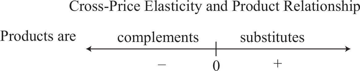
Figure 18
The elasticity of supply measures the responsiveness of the quantity supplied to price changes. The law of supply tells us that higher prices lead to larger quantities being supplied (supply curves slope upward), so the elasticity of supply should be positive. The formula for this elasticity is identical to that for demand elasticity, except that “quantity demanded” is replaced with “quantity supplied.”

As with demand elasticity, when supply elasticity is greater than 1, supply is elastic, and if it is less than 1, supply is inelastic. In many cases the elasticity of supply will increase over time as producers are able to adjust their production processes to respond to changes in prices. If the price of radishes increases, there may be little that can be done to increase supply within a few weeks, but within a few months farmland that was used to produce carrots can be replanted with radishes and the supply will become more responsive to price. The supply curve for particular entertainers like Taylor Swift is perfectly inelastic (vertical), because there is only one Taylor Swift to supply, regardless of the price.
Let’s consider how the concepts of supply, demand, elasticity, and surplus work together in real life. Imagine a product with relatively elastic demand, such as over-the-counter painkillers. There are many substitute brands producing them, and they aren’t absolutely necessary (minor aches and pains usually fade with time). As a result, demand for over-the-counter painkillers is relatively elastic, as illustrated by Figure 19.
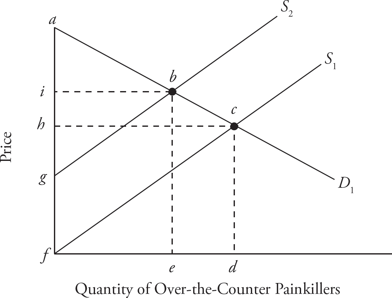
Figure 19
The initial supply and demand for over-the-counter painkillers are illustrated by S1 and D1. Suppose there is an environmental catastrophe, and one of the ingredients for over-the-counter pain killers becomes more expensive, causing the supply curve to shift inward. This shift is illustrated by S2. As a result, the equilibrium price increases from h to i, and the quantity demanded decreases from d to e. The change in total revenue is reflected by the difference between areas HCDF and IBEF. Consumer surplus shifts from areas ACH to ABI. Producer surplus shifts from areas HCF to IBG. Note that the changes in both consumer and producer surplus are relatively proportionate to the change in supply.
Now consider a product with relatively inelastic demand, such as opioid painkillers. There are few substitutes, and opioids are highly addictive, causing people to feel as though they are life dependent. As a result, the demand curve for opioids is relatively inelastic, as illustrated by Figure 20.

Figure 20
The initial supply and demand for opioids are illustrated by S1 and D1. Suppose another environmental catastrophe strikes, this time limiting opioid production. As a result, the supply curve shifts inward to S2. Notice the change in price, from h to i, and the adjusted total revenue IBEF.
Due to the inelasticity of the demand curve, the change in supply affects opioids differently than over-the-counter painkillers. For opioids, the reduction in quantity, from d to e, is less than over-the-counter painkillers, and the increase in price, from h to i, is greater than for over-the-counter painkillers. Due to the inelasticity of the demand curve, there is a greater change in price and total revenue for opioids per percent change in supply than for over-the-counter painkillers.
The effect of elasticity can also be seen in consumer surplus. While consumer surplus is illustrated by area ABI in Figure 19, the corresponding point A for opioids can’t be captured within the confines of Figure 20 because the demand curve is so steep. While consumer surplus is restricted in Figure 19, one can imagine that in a situation of perfect inelasticity, consumer surplus approaches infinity because the demand curve never intersects with the y-axis. In this way, both elasticity and consumer surplus model consumer behavior. The slope of the demand curve models consumer sensitivity to price, and consumer surplus models the utility buyers experience beyond the cost they paid for the good.
The demand for factors of production such as land, labor, and capital is derived from the demand for the products they produce. For example, if the demand for ice cream increases, the demand for ice cream ingredients will also increase.

Figure 21
If the demand for ice cream increases as illustrated on the left side of Figure 21, the price of ice cream—the value of the output of ice cream machines—will increase. Thus, the demand for such machines (a form of capital) will increase as illustrated on the right side of Figure 1.
The most that firms would be willing to pay for additional factors of production is determined by the value of each factor’s contribution to the production process. If a fourth bagel baker in a price-taking bagel shop would increase bagel production by 10 bagels per hour and bagels sell for $0.50 each, the most the bagel shop would pay for another baker is 10 × $0.50 = $5.00 per hour. In the language of economics, the marginal product of labor here is 10, the marginal revenue is $0.50, and the marginal revenue product of labor (MRPL) is $5.00. More generally
MRPL = MPL × Poutput
The fourth baker will be hired if the wage is less than $5.00 per hour. (If the wage is exactly $5.00 per hour, the shop is indifferent toward hiring the worker or not.)
Firms with market power face downward-sloping demand curves and are not price takers. In order to sell the additional output produced by additional units of an input, firms with downward-sloping demand curves must lower their prices on all units sold (assuming they cannot price-discriminate). Thus, the marginal revenue from each additional unit of output is not the price, but the price minus the losses on units previously sold at a higher price. The most such a firm would be willing to pay for another worker in the short run is again the MRPL.
The “L” for labor in the MRPL equation could be replaced with any other factor of production to establish the marginal revenue product formula for that factor. The MRPL curve represents the demand curve for either type of firm when only one factor of production is variable. In the long run when capital (for example) is variable in addition to labor, changes in the amounts of capital among other factors of production can affect the MPL and thus the MRPL and result in a labor demand curve that differs from the MRPL curve.
The MRPL curve slopes downward due to diminishing marginal returns, as explained above.
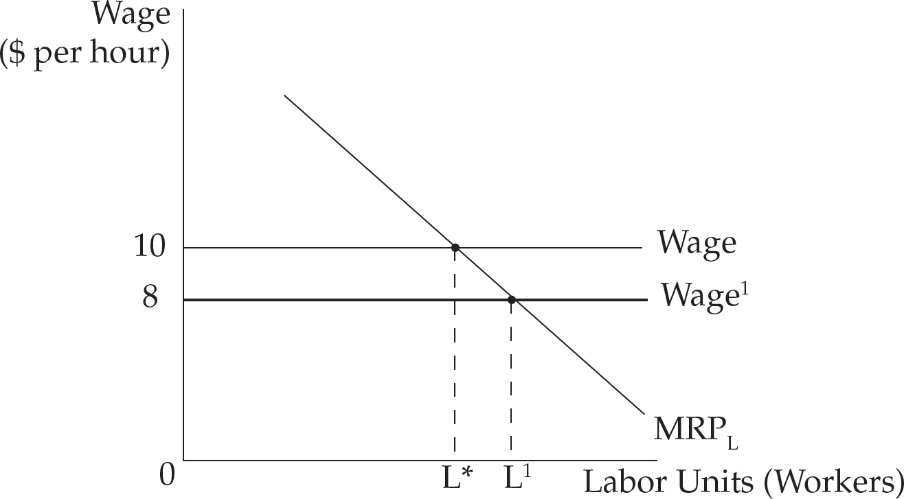
Figure 22
If the wage is $10 per hour as illustrated in Figure 22, the optimal quantity of labor to hire (L*) is found on the labor axis directly below the intersection, between the wage line and the MRPL line. If fewer than L* workers are hired, there is an opportunity to hire more workers and pay them less than the value of their contribution to revenues. If more than L* workers are hired, those in excess of L* are paid more than the value of their contribution to revenues and the firm would increase profits or decrease losses by cutting labor back to L*.
If the wage fell to $8, it would then be beneficial to hire those workers with marginal revenue products between $8 and $10; a total of L1 workers should be hired. If MRPL increased, as it would if the price of output increased or the marginal product of workers increased (for example, due to better training or technology), the demand for labor would shift to the right and more workers would be hired at any given wage. Decreases in MRPL would similarly shift the labor demand to the left.
As in the previous section, labor will be used here as an example in the explanation of factor markets. The determination of other factor prices is analogous.
In a perfectly competitive labor market, each firm is a wage taker, just as firms are price takers in a perfectly competitive output market. The market demand for labor is the sum of the firm demand curves. Market demand will thus increase or decrease in response to changes in the number of firms or the MRPL in the individual firms. The market supply of labor is the sum of all of the individual labor supply curves, and thus depends on the number of workers in the market and each worker’s willingness to provide labor services at various wage rates. Figure 23 illustrates labor market supply and demand curves on the right, and the horizontal labor supply confronting a competitive firm on the left.
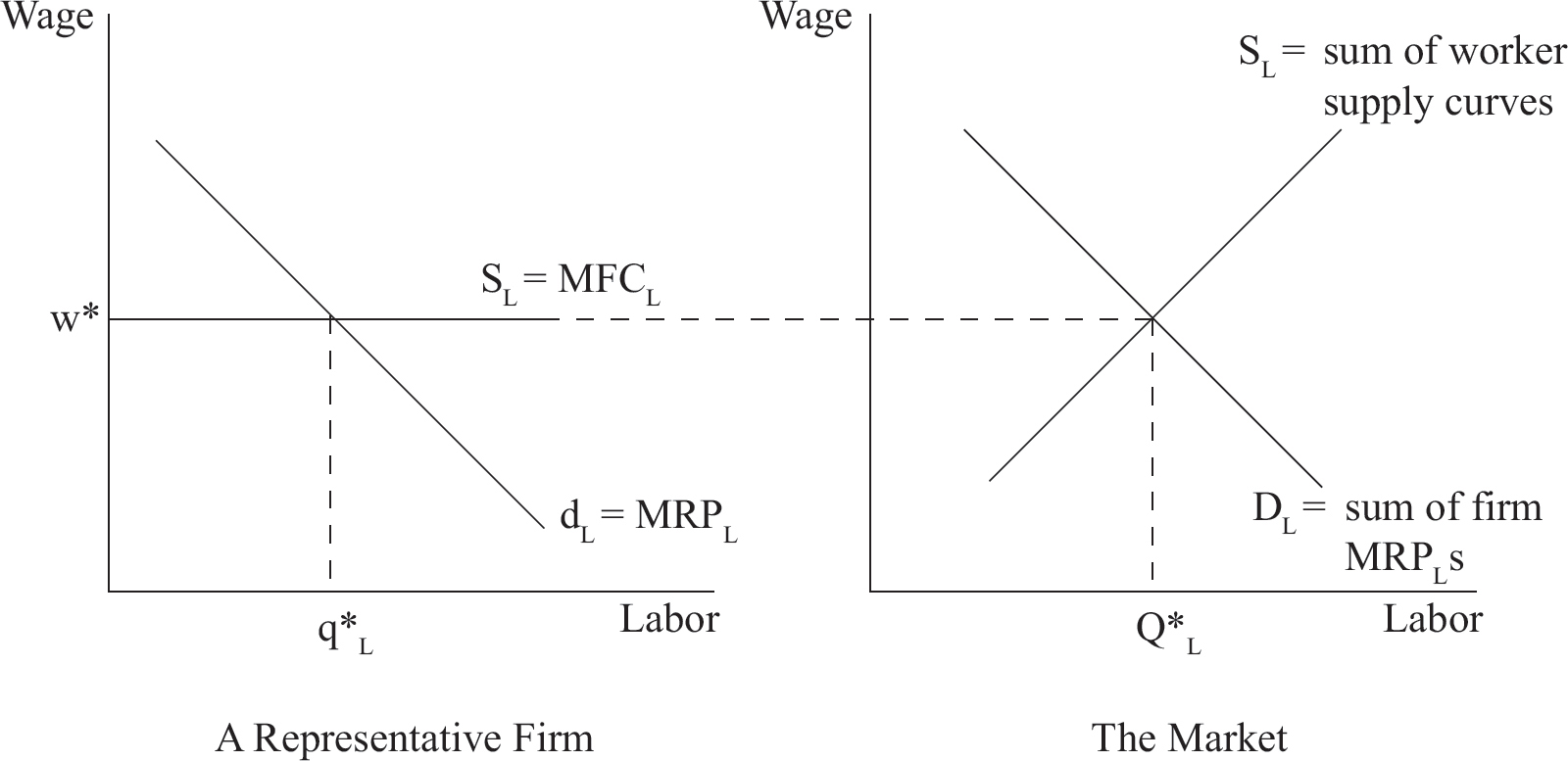
Figure 23: A Perfectly Competitive Labor Market
The intersection of the labor market demand and supply curves establishes the equilibrium wage. At this wage, everyone who would like to work has the opportunity to do so, meaning that there is no unemployment in this market. As described above, legislation that sets a minimum wage above the market equilibrium can act as a price floor for labor and cause unemployment. We will discuss unemployment further in the review of macroeconomic concepts.
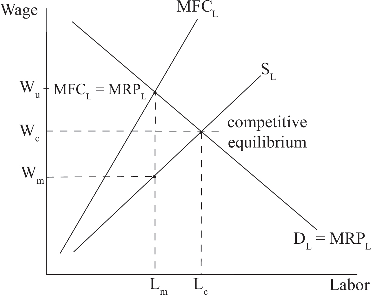
Figure 24: Monopsony
When one firm is the sole purchaser of labor services in a market, as a mining company might be in a small mining town, this firm is called a monopsony. Recall that marginal revenue is below price for a monopoly because it faces a downward-sloping market demand curve and must lower its price on all units sold in order to sell more. Similarly, a monopsony faces the entire upward-sloping labor supply curve as in Figure 24 and must raise wages to hire more workers. This results in a marginal factor cost or MFC (the additional cost of hiring one more worker) that is above the wage. For example, suppose a firm employing three workers for $10 per hour must pay $12 per hour to attract a fourth worker. The marginal factor cost of the fourth worker per hour is $12 plus the additional $2 per hour it must pay each of the first three workers to bring their wages from $10 to $12. The MFC is thus $12 + $2 + $2 + $2 = $18. Firms in a competitive labor market are wage takers, and their marginal factor cost equals the wage because they can hire all the workers they want at the same market wage.
A monopsony chooses the employment level at which MRPL = MFCL, indicated by Lm in Figure 24. The lowest wage the firm can pay to attract Lm workers, Wm, is determined by the labor supply curve directly above Lm. Notice that relative to the competitive labor market wage (Wc) and quantity of workers (Lc), the monopsony hires fewer workers and pays them less.
Workers in many industries increase their collective bargaining and lobbying strengths by forming labor unions. Unions use three general methods to increase the wages for their members. They attempt to
increase the demand for labor
decrease the supply of labor
negotiate higher wages
Because the demand for labor is derived from the demand for the products labor produces, one way to increase labor demand is to increase product demand. This is accomplished with calls for consumers to “look for the union label,” to lobby for favorable regulations and government expenditures, and to support protective tariffs and quotas that impede foreign competition.
Featherbedding agreements require employers to hire union members for particular tasks whether they are needed or not. Although the Taft-Hartley Act attempted to outlaw featherbedding and similar “make-work” agreements, the Supreme Court has permitted payments for nonproductive work. Examples include unnecessarily large minimum crew sizes on trains, and agreements that theaters will pay union musicians for performances even when orchestras from out of town are brought in to play.
Using an approach called exclusive unionism, some craft unions such as plumbers and electricians attempt to increase wages by restricting the supply of workers with their skills. When employers agree to hire only union workers, restricting the labor supply is as simple as restricting union membership. In other situations, unions can reduce the labor supply by lobbying for child labor laws, immigration restrictions, compulsory retirement, and occupational licensing.
For unskilled and semiskilled workers, it makes less sense to form an exclusive union because there are many available workers who could provide the same services. Instead, these groups tend to form inclusive or industrial unions that encourage as many workers as possible to join. Industrial unions try to use their size to their advantage when negotiating wage floors and compensation packages. On average, union members earn about 18 percent more than nonunionized workers in similar positions.
A monopoly exists when there is only one seller and a monopsony exists when there is only one buyer. A situation in which there is just one seller and one buyer in the same market, is called a bilateral monopoly. Because a union acts as a single seller of labor, and there are many industries dominated by a small number of employers that hire labor, situations resembling bilateral monopolies are not uncommon.
According to Figure 24, the monopsony desires to hire Lm workers and pay them Wm. The union will seek a wage of Wu, which is the marginal revenue product of the last worker hired (the MRP is what the last worker is worth to the employer, and the employer will most likely not pay workers more than what they are worth). Unlike the simple monopoly and monopsony situations, theory cannot predict the final wage in a bilateral monopoly. This will depend on the relative bargaining skills and strengths of the union and employer involved.
change in quantity demanded
change in demand
determinants of demand (TRIBE)
tastes and preferences
substitutes
complements
normal goods
inferior goods
marginal utility
total utility
consumer surplus
producer surplus
elasticity
price elasticity of demand
determinants of demand elasticity
(PAID)
elastic
luxury
necessity
unit elastic
inelastic
elasticity of supply
income elasticity of demand
normal goods
inferior goods
cross-price elasticity of demand
complements
substitutes
marginal revenue product of labor
wage taker
monopsony
marginal factor cost (marginal resource cost)
unions
featherbedding agreements
bilateral monopoly
See Chapter 9 for answers and explanations.
1. Which of the following could have caused an increase in the demand for ice cream cones?
(A) A decrease in the price of ice cream cones
(B) A decrease in the price of ice cream, a complimentary good to ice cream cones
(C) An increase in the price of ice cream, a complimentary good to ice cream cones
(D) A decrease in the price of lollipops, a close substitute for ice cream
(E) An increase in the supply of ice cream cones
2. The total utility from sardines is maximized when they are purchased until
(A) marginal utility is zero
(B) marginal benefit equals marginal cost
(C) consumer surplus is zero
(D) distributive efficiency is achieved
(E) deadweight loss is zero
3. If a 3 percent increase in price leads to a 5 percent increase in the quantity supplied
(A) supply is unit elastic
(B) demand is inelastic
(C) demand is elastic
(D) supply is elastic
(E) supply is inelastic
4. Normal goods always have a/an
(A) elastic demand curve
(B) inelastic demand curve
(C) elastic supply curve
(D) negative income elasticity
(E) positive income elasticity
5. When the cross-price elasticity of demand is negative, the goods in question are necessarily
(A) normal
(B) inferior
(C) complements
(D) substitutes
(E) luxuries
6. If a business wants to increase its revenue and it knows that the elasticity quotient of demand of its product is equal to 0.78, it should
(A) decrease price because demand is elastic
(B) decrease price because demand is unit elastic
(C) decrease price because demand is inelastic
(D) increase price because demand is inelastic
(E) increase price because demand is elastic
7. A student eats 3 slices of pizza while studying for his Economics exam. The marginal utility of the first slice of pizza is 10 utils, the second slice is 7 utils, and the third slice is 3 utils. Which of the statements below holds true with the above data?
(A) The student would not eat any more pizza.
(B) The marginal utility of the fourth slice of pizza will be 0.
(C) The student should have stopped eating pizza after 2 slices.
(D) The total utility this student received from eating pizza is 20 utils.
(E) The total utility decreases after the first slice of pizza because of diminishing marginal utility.
8. Relative to a competitive input market, a monopsony
(A) pays less and hires more workers
(B) pays less and hires the same number of workers
(C) pays more and hires more workers
(D) pays more and hires fewer workers
(E) pays less and hires fewer workers
9. Which of the following is NOT among the methods unions use to increase wages?
(A) Negotiations to obtain a wage floor
(B) Restrictive membership policies
(C) Efforts to decrease the prices of substitute resources
(D) Featherbedding or make-work rules
(E) Efforts to increase the demand for the product they produce
10. A bilateral monopoly exists when
(A) a monopsony buys from a monopoly
(B) a monopoly sells to two different types of consumers
(C) a monopoly buys from a monopsony
(D) a monopolist sells two different types of goods
(E) a monopoly sells at two different prices
The demand curve shifts with
Tastes and preferences of consumers
the prices of Related goods
the Income of buyers
the number of Buyers
Expectations for the future
Marginal utility is the additional utility gained from consuming one more unit of a good.
Total utility is the sum of all marginal utility values gained from each unit consumed.
Consumer surplus is the value a buyer receives from the purchase of a good in excess of what the consumer pays for it; producer surplus is the difference between the price a seller receives for a good and the minimum price for which she would be willing to supply a quantity of the good.
The price elasticity of demand for a given good describes the extent to which consumer behavior will change as the price of the good changes.
The elasticity of a good relates to
the Proportion of the consumer’s income spent on the good
the Availability of close substitutes
the Importance of a good
the ability to Delay the purchase of a good
A good is elastic (a luxury) if %ΔQd > %ΔP
A good is unit elastic if %ΔQd = %ΔP
A good is inelastic (a necessity) if %ΔQd < %ΔP
Knowing the elasticity of a demand curve tells sellers how much their total revenue will change with a change in price:
elastic goods: P
 TR
TR
unit elastic goods: PTR constant
inelastic goods: PTR
The elasticity of supply measures the responsiveness of the quantity supplied to price changes.
Elasticity of supply is calculated by 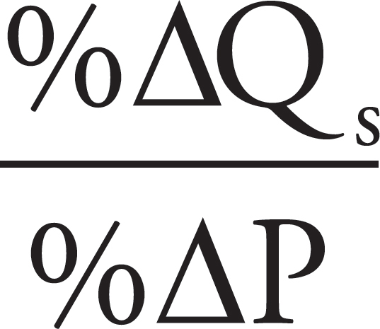
Income elasticity of demand measures the responsiveness of the quantity demanded to changes in income.
Income elasticity is calculated by 
Individuals buy more normal goods (positive income elasticity) when their income increases; they buy more inferior goods (negative elasticity) when their income decreases.
The cross-price elasticity of demand measures the responsiveness of the quantity demanded of one good to the price of another.
Cross-price elasticity of good x in relation to good y is calculated by 
When cross-price elasticity is negative, then goods x and y are complements; when cross-price elasticity is positive, then goods x and y are substitutes.
The marginal revenue product of labor is the amount of revenue generated by one additional unit of labor; calculate using this formula:
MRPL = MPL × Poutput
The above equation can be used for any of the factors of demand.
A monopsony occurs when one firm is the sole purchaser of labor services.
The marginal factor cost (MFC) is the additional cost of one more unit of labor.
A monopsony will choose an employment level at which MRPL = MFCL.
Workers increase their collective bargaining and lobbying strengths by forming labor unions. They attempt to
increase the demand for labor
decrease the supply of labor
negotiate higher wages
A bilateral monopoly occurs when there is only one buyer and one seller in the market.