3 Searching

The fact that algorithms can do all sorts of stuff, from translating text to driving cars, can give us a misleading picture of what algorithms are mostly used for. The answer may seem mundane. It is unlikely that you will be able to find any computer program doing anything at all useful without employing algorithms for searching in data.

That is because searching in one form or another appears in almost every context. Programs take in data; often they will need to search for something in them and so a searching algorithm will almost certainly be used. Not only is searching a frequent operation in programs but, because it happens frequently, searching can be the most time-consuming operation in an application. A good search algorithm can result in dramatic improvements in speed.

A search involves looking for a particular item among a group of items. This general problem description encompasses several variations. It makes a big difference whether the items are ordered in some way that is related to our search or come in random order. A different scenario occurs when the items are given to us one by one and we have to decide if we have found the correct one right when we confront it, without the ability to rethink our decision. If we search repeatedly in a set of items, it is important to know if some items are more popular than others so that we end up searching for them more often. We will examine all these variations in this chapter, but keep in mind that there are more. For example, we will only present exact search problems, but there are many applications in which we need an approximate search. Think of spellchecking: when you mistype something, the spellchecker will have to search for words that are similar to the one it fails to recognize.

Searching in one form or another appears in almost every context. . . . A good search algorithm can result in dramatic improvements in speed.

As the data volumes increase, the ability to search efficiently in a huge number of items has become more and more significant. We’ll see that if our items are ordered, the search can scale extremely well. In chapter 1 we stated that it is possible to find something among a billion sorted items in about 30 probes; now we will see how this can be actually done.

Finally, a search algorithm will give us a glimpse of the dangers that lurk when we move from an algorithm to an actual implementation in a computer program, which has to run within the confines of a particular machine.

A Needle in a Haystack

The simplest way to search is what we do to find the proverbial needle in a haystack. If we want to find something in a group of objects and there is absolutely no structure in them, then the only thing we can do is to check one item after the other until we either find the item we are looking for or fail to find it after exhausting all items.

If you have a deck of cards and are looking for a particular one in them, you can start taking off the cards from the top of the deck until you find the one you are looking for or run out of cards. Alternatively, you can start taking off the cards one by one from the bottom of the deck. You can even take off cards from random positions in the deck. The principle is the same.

Usually we do not deal with physical objects in computers but rather digital representations of them. A common way to represent groups of data on a computer is in the form of a list. A list is a data structure that contains a group of things in such a way that from one item we can find the next one. We can usually think of the list as containing linked items, where one item points to the next one, until the end, where the last item points to nothing. The metaphor is not far from the truth because internally the computer uses memory locations to store items. In a linked list, each item contains two things: its payload data and the memory location of the next item on the list. A place in memory that holds the memory location of another place in memory is called a pointer. Therefore in a linked list, each element contains a pointer to the next element. The first item of a list is called its head. The items in a list are also called nodes. The last node does not point to anywhere; we say that it points to null: nothingness on a computer.

A list is a sequence of items, but it is not necessary that the sequence is ordered using some specific criterion. For example, the following is a list containing some letters from the alphabet:

If we have an unordered list, the algorithm for finding an item on it goes like this:

1. Go to the head of the list.
2. If the item is the one we are looking for, report that it is found and stop.
3. Go to the next item on the list.
4. If we are at null, report that the search item was not found and stop. Otherwise, return to step 2.

This is called a linear or sequential search. There is nothing special about it; it is a straightforward implementation of the idea of examining each single thing in turn until we find the one we want. In reality, the algorithm makes the computer jump from pointer to pointer until it either reaches the item we are looking for or null. Below we show what is happening when we search for E or X:

If we search among n items, the best thing that can happen is to hit on the item we want immediately, which will occur if it is the head of the list. The worst thing that can happen is that the item is the last one on the list or not on the list at all. Then we must go through all n items. Therefore the performance of sequential search is .

There is nothing we can do to improve on that time if the items appear on the list in a random sequence. Going back to a deck of cards, you can see why this is so: if the deck is properly shuffled, there is no way to know in advance where we’ll find our card.

Sometimes people have trouble with that. If we are looking for a paper among a large pile, we may tire of going one after the other. We may even think of how unlucky we would be should the paper turn out to be at the bottom of the pile! So we stop going through the pile in order and peek at the bottom. There is nothing wrong in peeking at the bottom, but it’s wrong to think that this improves our chances of finishing the search quickly. If the pile is random, then there is no reason why the sought-after item is not the first, last, or one right in the middle. Any position is equally likely, so starting from the top and making our way to the bottom of the pile is as good a strategy as any other that ensures we examine each item exactly once. It is usually simpler to keep track of what we looked at if we work in a specific order, however, than jumping around erratically, and that’s why we prefer to stick with a sequential search.

All this holds as long as there is no reason to suspect that the search item is in a particular position. But if this is not true, then things change, and we can take advantage of any extra information we may have to speed up our search.

The Matthew Effect and Search

You may have noticed that in an untidy desk, some things find their way to the top of the pile, while some others seem to slip to the bottom. When finally cleaning up the mess, the author has had the pleasant experience of discovering buried deep down in a heap things he believed were long lost. The experience has probably occurred to others as well. We tend to place things we use frequently close; things we have little use for slip further and further out of reach.

Suppose we have a pile of documents on which we need to work. The documents are not ordered in any way. We go through the pile, searching for the document we need, processing it, and then placing it not where we found it but instead on the top of the pile. Then we go again with our business.

It may happen that we do not work with the same frequency on all documents. We may return to some of them again and again, while we may only rarely visit others. If we continue placing every document on the top of the pile after working on it, after some time we’ll find out that the most popular documents will be near the top, while the ones we accessed the least often will have moved toward the bottom. This is convenient for us because we spend less time locating the frequently used documents and thus less time overall.

This suggests a general searching strategy, where we search for the same items repeatedly, and some items are more popular than others. After finding an item, bring it forward so that we’ll be able to find it faster the next time we will look for it.

How applicable would such a strategy be? It depends on how often we observe such differences in popularity. It turns out that they happen a lot. We know the saying “the rich get richer, and the poor get poorer.” It is not just about rich and poor people. The same thing appears to a bewildering array of aspects in different fields of activity. The phenomenon has a name, the Matthew effect, after the following verse in the Gospel of Matthew (25:29): “For unto every one that hath shall be given, and he shall have abundance: but from him that hath not shall be taken away even that which he hath.”

The verse talks about material goods, so let’s think about wealth for a minute. Suppose you have a large stadium, capable of holding 80,000 people. You are able to measure the average height of the people in the stadium. Your result may be something around 1.70 meters (5 feet, 7 inches). Imagine that you take out somebody randomly from the stadium and put in the tallest person in the world. Will the average height differ? Even if the tallest person is 3 meters tall (no such height has ever been recorded), the average height would remain stuck at its previous value—the difference with the previous average being less than a tenth of a millimeter.

Imagine now that instead of measuring the average height, you measure the average wealth. The average wealth of your 80,000 people could be $1 million (we are assuming a wealthy cohort). Now you substitute again somebody inside with the richest person in the world. That person could have a wealth of $100 billion. Would this make a difference? Yes, it would—and a big one. The average would increase from $1 million to $2,249,987.5, or more than double. We are aware that wealth is not distributed equally around the world, but we may not be aware of how unequal the distribution is. It is much more unequal than a distribution of natural measures like height.

The same difference in endowments occurs in many other settings. There are many actors you have never heard of. And there are a few stars who have appeared in many movies, earning millions of dollars. The term “Matthew effect” was coined by the sociologist Robert K. Merton in 1968, when he observed that famous scientists get more credit for their work over their lesser-known colleagues, even if their contributions are similar. The more famous scientists are, the more famous they will get.

Words in a language follow the same pattern: some of them are much more popular than others. The list of domains that are characterized by such jarring inequalities includes the size of cities (megacities are many times larger than the average city) and number, links, and popularity of web sites (most sites are honored only by the occasional visitor, while others rake in millions). The prevalence of such unequal distributions, where a few elements of a population obtain a disproportionate amount of resources, has been a rich field of inquiry over the last few years. Researchers are looking into the reasons and laws that underlie the emergence of such phenomena.1

It is possible that the items in which we are searching exhibit such differences in popularity. Then a search algorithm that will take advantage of the varying popularity of the search items can work much like putting each document that we find at the top of the pile:

1. Search for the item using a sequential search.
2. If the item is found, report that it is found, put it at the front of the list, at its head, and stop.
3. Otherwise, report that the item was not found and stop.

In the following figure, finding E on the list will bring it to the front:

A possible criticism of this move-to-front algorithm is that it will promote to the front even an item that we only rarely search for. That is true, but if the item is not popular, it will gradually move toward the end of the list as we search for other items because these items will move to the front. We can take care of the situation, however, by adopting a less extreme strategy. Instead of moving each item we find bang to the front, we can move it just one position forward. This is called the transposition method:

1. Search for the item using a sequential search.
2. If the item is found, report that it is found, exchange it with the previous one (if it is not the first one), and stop.
3. Otherwise, report that the item was not found and stop.

In this way, items that are popular will gradually make their way to the front, and less popular items will move to the back, without sudden upheavals.

Both the move-to-front and transposition methods are examples of a self-organizing search; the name comes because the list of items is organized as we go with our searches and will reflect the popularity of the searched items. Depending on how the popularity ranges among items, the savings can be significant. While with a sequential search we can expect a performance of , a self-organizing search with the move-to-front method can attain a performance of . If we have about a million items, this is the difference between 1 million and about 50,000. The transposition method can have even better results, but it requires more time to achieve them. That’s because both methods require a “warm-up period” in which popular items will show themselves up and make their way to the front. In the move-to-front method, the warm-up is short; in the transposition method, the warm-up takes longer, but then we get better results.2

Kepler, Cars, and Secretaries

After the celebrated astronomer Johannes Kepler (1571–1630) lost his wife to cholera in 1611, he set out to remarry. A methodical man, he did not leave things to chance. In a long letter to a Baron Strahlendorf, he describes the process he followed. He planned to interview 11 possible brides before making his decision. He was strongly attracted to the fifth candidate, but was swayed against her by his friends, who objected to her lowly status. They advised him to reconsider the fourth candidate instead. But then he was turned down by her. In the end, after examining all 11 candidates, Kepler did marry the fifth one: 24-year-old Susanna Reuttinger.

This little story is a stretched example of a search; Kepler was searching for an ideal match, among a pool of possible candidates. Yet there was a kink in the process that he was probably not aware of when he started: it might not be possible to go back to a possible match after he had rejected it.

We can recast the problem in more contemporary terms, as looking for the best way to decide which car to buy. We have decided beforehand that we will visit a certain number of car dealerships. Also, our amour propre will not allow us to return to a car dealership after we have walked away from it. If we have declined a car, saving face is paramount, so that we cannot go back and say that we changed our mind. Or perhaps somebody else walked in and bought the car after we left. Be it as it may, we have to make a final decision at each dealership, to buy the car or let go, and not come back.

This is an instance of an optimal stopping problem. We have to take an action, while trying to maximize a reward or minimize a cost. In our example, we want to decide to buy the car, when this decision will result in the best car we can buy. If we decide too early, we may settle on a car that is worse than a car we have not seen yet. If we decide too late, we may discover to our chagrin that we saw, but missed, the best car. When is the optimal time to stop and make a decision?

The same issue is usually described in a more callous way as the secretary problem. You want to select a secretary from a pool of candidates. You can interview the candidates one by one. You must make a decision to hire or not at the end of each interview, however. If you reject a candidate, you cannot later change your mind and make an offer (the candidate might be too good and thus be snapped by somebody else). How will you pick the candidate?

There is a surprisingly simple answer. You go through the first 37 percent of the candidates, rejecting them all, but keeping a tab on the best one among them as your benchmark. The number 37, which seems magical, occurs because , where e is Euler’s number, approximately equal to 2.7182 (we saw Euler’s number in chapter 1). Then you go through the rest of the candidates. You stop at the first of the rest that is better than your benchmark. That will be your pick. In algorithmic form, if you have n candidates:

1. Calculate , to find the 37 percent of the n candidates.
2. Examine and reject the first candidates. You will use the best one among them as a benchmark.
3. Continue with the rest of candidates. Pick the first one that is better than your benchmark, and stop.

The algorithm will not always find the best candidate; after all, the best candidate overall may be the benchmark candidate you identified in the first 37 percent, and that you have rejected. It can be proved that it will find the best candidate in 37 percent (again, ) of all cases; moreover, there is no other method that will manage to find the best candidate in more cases. In other words, the algorithm is the best you can do: although it may fail to give you the best candidate in 63 percent of the cases, any other strategy you may decide to follow will fail in more cases than that.

Going back to cars, suppose we decide to visit 10 car dealerships. We should visit the first four and take note of the best offer by these four, without buying. Then we start visiting the remaining six dealerships and we’ll buy from the first dealership that gives us an offer better than the one we noted down (we’ll then skip the rest). We may discover that all six dealerships make worse offers then the first four that we visited without buying. But no other strategy can give us better odds of getting the best deal.

We have assumed that we want to find the best possible candidate and will settle for nothing less. But what if we can in fact settle for something less? That means that even though ideally we would want the best secretary or car, we can make do with another choice, with which we may be happy, although not as happy had we picked up the best. If we frame the problem like that, then the best way to make our selection is to use the same algorithm as above, but examining and discarding the square root, , of the candidates. If we do that, the probability that we will make the best choice increases with the number of candidates: as n increases, the probability that we’ll pick the best goes to 1 (that is, 100 percent).3

Binary Search

We have considered different ways to search, corresponding to different scenarios. A common thread in all these was that the items that we examine are not given to us in any specific order; at best, we order them gradually by popularity in a self-organized search. The situation changes completely if the items are ordered in the first place.

Let’s say we have a pile of folders, each one of which is identified by a number. The documents in the pile are ordered according to their identifier, from the lowest to highest number (there is no need for the numbers to be consecutive). If we have such a pile and are looking for a document with a particular identifier, it is foolish to start from the first document and make our way to the last until we find the one we are looking for. A much better strategy is to go straight to the middle of the pile. Then we compare the number identifier on the document in the middle to the number of the document that we are looking for. There are three possible outcomes:

1. If we are lucky, we may have landed exactly on the document that we want. We are done; our search is over.
2. The identifier of the document we are looking for is greater than the identifier of the document we have in our hands. Then we know for sure that we can discard the document at hand as well as all preceding documents. As they are ordered, they will all have smaller identifiers. We have undershot our target.
3. The opposite happens: the identifier of the document we are looking for is smaller than the identifier of the document we have in our hands. Then we can safely discard the document at hand as well as all the documents that come after it. We have overshot our target.

In either of the last two outcomes, we are now left with a pile that is at most half the original one. If we start with an odd number of documents, say n, splitting n documents in the middle gives us two parts, each with items (discarding the fractional part in the division):

With an even number of items, splitting them will give us two parts, one with items and another one with items:

We have still not found what we were looking for, but we are much better than before; we have much fewer items to go through now. And so we do. We check the middle document of the remaining items and repeat the procedure.

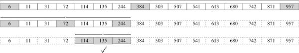
In the figure on the following page, you can see how the process evolves for 16 items, among which we are looking for item 135. We mark out the boundaries inside which we search and the middle item with gray.

In the beginning, the domain of our search is the full set of items. We go to the middle item, which we find out is 384. This is bigger than 135, so we discard it, along with all the items to its right. We take the middle of the remaining items, which turns out to be 72. This is smaller than 135, so we discard it, along with all the items on its left. Our search domain has shrunk to just three items. We take the middle one and find that it is the one we want. It took us only three probes to finish our search, and we did not even need to check 13 of the 16 items.

The process will also work if we are looking for something that does not exist. You can see that in the next figure, where we are searching among the same items for one labeled 520.

This time, 520 is greater than 384, so we restrict our search to the right half of the items. There we find that the middle of the upper half is 613, greater than 520. Then we limit our search to just three items, the middle of which is 507. This is smaller than our target of 520. We discard it and now are left with only one item to check, which we discover is not the one we want. So we can finish our search reporting that it was unsuccessful. It took us only four probes.

The method we described is called binary search because each time we cut in half the domain of values in which we search. We call the domain of values where we perform our search the search space. Using this concept, we can render the binary search as an algorithm comprising these steps:

1. If the search space is empty, we have nowhere to look, so report failure and stop. Otherwise, find the middle element of the search space.
2. If the middle element is less than the search term, limit the search space from the middle element onward and go back to step 1.

3. Otherwise, if the middle element is greater than the search term, limit the search space up to the middle element and go back to step 1.
4. Otherwise, the middle element is equal to the search term; report success and stop.

In this way, we divide by two the items that we have to search. This is a divide-and-conquer method. It results in repeated division, which as we have seen in chapter 1 gives us the logarithm. Repeated division by two gives us the logarithm base two. In the worst case, a binary search will keep dividing and dividing our items, until it cannot divide any further, like we saw in the unsuccessful search example. For n items, this cannot happen more than times; it follows that the complexity of a binary search is .

The improvement compared to a sequential search, even a self-organized search, is impressive. It will not take more than 20 probes to search among a million items. Viewed from another angle, with a hundred probes we are able to search and find any item among , which is more than one nonillion.

The efficiency of a binary search is astounding. Its efficiency is probably only matched by its notoriety. It is an intuitive algorithm. But this plain method has proved time and again tricky to get right in a computer program. For reasons that have nothing to do with the binary search algorithm per se, but rather the way we turn algorithms into real computer code in programming language, programmers have been prey to insidious bugs that have crept into their implementations. And we are not talking about rookies; even world-class programmers have failed to get it right.4

To get an idea of where such bugs may lurk, consider how we find the middle element among the items we want to search in the first step of the algorithm. Here is a simple idea: the middle element of the mth and nth elements is , rounded if the result is not a natural number. This is true, and it follows from elementary mathematics, so it applies everywhere.

Except in computers. Computers have limited resources, memory among them. It is not possible, therefore, to represent all the numbers we want on a computer. Some numbers will simply be too big. If the computer has an upper limit on the size of the numbers that it can handle, then both m and n should be below that limit. Of course, is below that limit. But to calculate , we have to calculate and then divide it by two, and that sum may be larger than the upper limit! This is called overflow: going beyond the range of allowable values. So you get a bug that you had never thought would bite you. The result will not be the middle value but instead something else entirely.

Do not despair if you find yourself wretched poring over a line of code that does not do what you think it should do. You are not unique. It happens to all; it happens to the best.

Once you know about it, the solution is straightforward. You do not calculate the middle as but rather . The result is the same, but no overflow occurs. In retrospect it seems simple. In hindsight, though, everybody is a prophet.

We are interested in algorithms, not programming, here, but let the author share a bit of advice for those who write or want to write computer programs. Do not despair if you find yourself wretched poring over a line of code that does not do what you think it should do. Do not be dismayed if the following day you realize that, indeed, the bug was before your eyes all the time. How could you have failed to see it? You are not unique. It happens to all; it happens to the best.

Binary search requires that the items should be sorted. So to reap its benefits, we should be able to sort items efficiently—which allows us to segue to the next chapter, where we’ll see how we can sort things with algorithms.