6
Deep Learning
Deep learning systems have burst onto the scene in recent years, often making headlines in mainstream media. There we see computer systems performing feats that were the purview of humans. Even more tantalizing is the fact that these systems are frequently presented as having some similarities to the way the human mind works—which of course cues to the idea that perhaps the key for artificial intelligence may be to mimic the workings of human intelligence.
Brushing aside the hype, most scientists working on deep learning do not ascribe to the view that deep learning systems work like the human mind. The goal is to exhibit some useful behavior, which we often associate with intelligence. We do not go about copying nature, however; in fact, the architecture of the human brain is much too complicated to emulate on a computer. But we do take some leaves out of nature’s book, simplify them a lot, and try to engineer systems that could, in certain fields, do things usually done by biological systems that have evolved over millions of years. Moreover, and this concerns us here in this book, deep learning systems can be understood in terms of the algorithms they employ. This will shed some light on what they do exactly, and how. And it should help us see that underneath their accomplishments, the main ideas are not complicated. That should not belittle the achievements of the field. We’ll see that deep learning requires an enormous amount of human ingenuity in order to come to fruition.
To understand what deep learning is about, we need to start small, from humble beginnings. On these we will build a more and more elaborate picture, until, at the end of the chapter, we will be able to make sense of what the “deep” in deep learning stands for.
Neurons, Real and Artificial
Our starting point will be the main building block of deep learning systems, which does come from biology. The brain is part of the nervous system, and the main components of the nervous system are cells called neurons. Neurons have a particular shape; they look different from the globular structures that we usually associate with cells. You can see below one of the first images of neurons, drawn in 1899 by the Spanish Santiago Ramón y Cajal, a founder of modern neuroscience.1
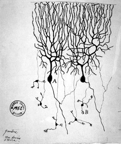
The two structures that stand out in the middle of the image are two neurons of the pigeon brain. As you can see, a neuron consists of a cell body and the filaments that extrude from it. These filaments connect a neuron to other neurons through synapses, embedding the neurons in a network. The neurons are asymmetrical. There are many filaments on the one side and one filament on the other side of each neuron. We can think of the many filaments on the one side as the neuron’s inputs, and the long outgoing filament on the other side as the neuron’s output. The neuron takes input in the form of electric signals from its incoming synapses and may send a signal to other neurons. The more inputs it receives, the more likely it is to output a signal. We say that the neuron then fires or is activated.
The human brain is a vast network of neurons, which number about one hundred billion, and each one of them is connected on average to thousands of other neurons. We do not have the means to build anything like that, but we can build systems out of simplified, idealized models of neurons. This is a model of an artificial neuron:

That is an abstract version of a biological neuron, being just a structure with a number of inputs and one output. The output of a biological neuron depends on its input; similarly, we want the artificial neuron to be activated depending on its input. We are not in the realm of brain biochemistry, but in the world of computing, so we need a computational model for our artificial neuron. We assume that the signals received and sent by neurons are numbers. Then the artificial neuron takes all its inputs, calculates some arithmetic value based on them, and produces some result on its output. We do not need any special circuit for implementing an artificial neuron. You can think of it as a small program inside a computer that takes its inputs and produces an output, much like any other computer program. We do not need to build artificial neural networks literally; we can and do simulate them.
Part of the learning process in biological neural networks is the strengthening or weakening of the synapses between neurons. The acquisition of new cognitive abilities and absorption of knowledge result in some synapses between neurons getting stronger, while others get weaker or even drop off completely. Moreover, synapses may not only excite a neuron to fire but also inhibit its activation; when a signal arrives on that synapse, the neuron should not fire. Babies have actually more synapses in their brains than adults. Part of growing up is pruning the neural network inside our heads. Perhaps we could think of the infant brain as a block of marble; as we go through the years in our lives, the block is chipped through our experiences and the things we learn, and a form emerges.
In an artificial neuron, we approximate the plasticity of synapses, their excitatory or inhibitory role, through weights we apply to the inputs. In our model artificial neuron, we have n inputs, ![]() ,
, ![]() , . . . ,
, . . . , ![]() . To each one of them we apply a weight,
. To each one of them we apply a weight, ![]() ,
, ![]() , . . . ,
, . . . , ![]() . Each weight is multiplied by the corresponding input. That final input received by a neuron is the sum of the products:
. Each weight is multiplied by the corresponding input. That final input received by a neuron is the sum of the products: ![]() . To this weighted input we add a bias b, which you can think of as the propensity the neuron has to fire; the higher the bias, the more likely it is to be activated, while a negative bias added to the weighted input will actually inhibit the neuron from firing.
. To this weighted input we add a bias b, which you can think of as the propensity the neuron has to fire; the higher the bias, the more likely it is to be activated, while a negative bias added to the weighted input will actually inhibit the neuron from firing.
The weights and bias are the parameters of the neuron because they influence its behavior. As the output of a biological neuron depends on its inputs, so the output of an artificial neuron depends on the input it gets. This happens by feeding the input into a special activation function, the result of which is the neuron’s output. This is what happens, diagrammatically, using ![]() as a stand-in for the activation function:
as a stand-in for the activation function:

The simplest activation function is a step function, giving us a result of 0 or 1. The neuron fires and outputs 1 if the input to the activation function is greater than 0, or stays silent outputting 0 otherwise:

Instead of a bias, it is helpful to think of a threshold. The neuron outputs 1 if the weighted input exceeds a threshold or outputs 0 otherwise. Indeed, if we write the behavior of the neuron as a formula, the first condition is ![]() or
or ![]() . By using
. By using ![]() , we get
, we get ![]() , where t, the opposite of the bias, is the threshold that the weighted input needs to pass for the neuron to fire.
, where t, the opposite of the bias, is the threshold that the weighted input needs to pass for the neuron to fire.
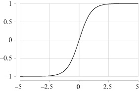
In practice we tend to use other, related activation functions instead of the step function. On the next page you can see three common ones.
The one on the top is called sigmoid because it has an S shape.2 Its output ranges from 0 to 1. A large positive input results in outputs close to 1; a large negative input results in an output close to 0. This approximates a biological neuron that fires on large inputs and stays silent otherwise, and is a smooth approximation to the step function. The activation function in the middle is called tanh, short for hyperbolic tangent (there are various ways to pronounce it: “tan-H,” “then,” or “thents” with a soft th, as in thanks).3 It looks like the sigmoid function, but it differs in that its output ranges from ![]() to
to ![]() ; a large negative input results in a negative output, mimicking an inhibitory signal. The function at the bottom is called a rectifier; it turns all negative inputs to 0, otherwise its output is directly proportional to its input. The following table shows the output of the three activation functions for different inputs.
; a large negative input results in a negative output, mimicking an inhibitory signal. The function at the bottom is called a rectifier; it turns all negative inputs to 0, otherwise its output is directly proportional to its input. The following table shows the output of the three activation functions for different inputs.


| -5 | -1 | 0 | 1 | 5 | |
|---|---|---|---|---|---|
|
sigmoid |
0.01 |
0.27 |
0.5 |
0.73 |
0.99 |
|
tanh |
-1 |
-0.76 |
0 |
0.76 |
+1 |
|
rectifier |
0 |
0 |
0 |
1 |
5 |
If you wonder why the proliferation of activation functions (there are also others), it is because it has been found in practice that particular activation functions are more suitable in some applications than others. As the activation function is crucial for the behavior of a neuron, neurons are often named by their activation functions. A neuron that uses the step function is called a Perceptron.4 Then we have sigmoid and tanh neurons. We also call neurons units, and a neuron using the rectifier is called a ReLU, for rectified linear unit.
A single artificial neuron can learn to distinguish between two sets of things. For example, take the data in the figure on the top of the next page, portraying a set of observations with two features, ![]() , on the horizontal axis, and
, on the horizontal axis, and ![]() , on the vertical axis. We want to build a system that will tell apart the two blobs. Given any item, the system will be able to decide whether the item falls in one group or another. In effect, it will create a decision boundary, like in the figure at the bottom. For any combination of
, on the vertical axis. We want to build a system that will tell apart the two blobs. Given any item, the system will be able to decide whether the item falls in one group or another. In effect, it will create a decision boundary, like in the figure at the bottom. For any combination of ![]() , it will tell us whether the item belongs to the lighter or darker group.
, it will tell us whether the item belongs to the lighter or darker group.


The neuron will have only two inputs. It will take each ![]() pair and calculate an output. If we are using the sigmoid activation function, the output will be between 0 and 1. We’ll take the values greater than 0.5 to fall into one group and the other values to fall into the other. In this way the neuron will act as a classifier, sorting our data into distinct classes. But how does it do that? How can the neuron get to the point of being able to classify data?
pair and calculate an output. If we are using the sigmoid activation function, the output will be between 0 and 1. We’ll take the values greater than 0.5 to fall into one group and the other values to fall into the other. In this way the neuron will act as a classifier, sorting our data into distinct classes. But how does it do that? How can the neuron get to the point of being able to classify data?
The Learning Process
At the moment of its creation, our neuron cannot recognize any kind of data; it learns to recognize them. The way it learns is by example. The whole process is akin to having a student learn something by giving them a large bunch of problems on a subject, along with their solutions. We ask the student to study each problem and its solution. If they are diligent, we expect that after the student has gone through a number of problems, they will have figured out how to get from a problem to its solution and will even be able to solve new problems, related to the ones they studied, but this time without having recourse to any solutions.
When we do this, we train the computer to find the solutions; the set of solved example problems is called the training data set. This is an instance of supervised learning because the solutions guide the computer, like a supervisor, toward finding the right answers. Supervised learning is the most common form of machine learning, the entire discipline that deals with methods where we train computers to do things. Apart from supervised learning, machine learning also encompasses unsupervised learning, where we provide the computer with a training data set, but not with any accompanying solutions. There are important applications of unsupervised learning, like, for example, grouping observations into different clusters (there is no a priori solution to what a correct cluster of observations is). In general, though, supervised learning is more powerful than unsupervised learning, as we provide more information during training. We will only deal with supervised learning here.
At the moment of its creation, our neuron cannot recognize any kind of data; it learns to recognize them. The way it learns is by example.
After training, the student often passes some tests to see how well they mastered the material. Similarly, in machine learning, after training we give the computer another data set that it has not seen before and ask it to solve this test data set. Then we evaluate the performance of the machine learning system based on how well it manages to solve the problems in the test data set.
In the classification task, training for supervised learning works by giving the neuron network a large number of observations (problems) along with their classes (solutions). We expect that the neuron will somehow learn how to get from an observation to its class. Then if we give it an observation it has not seen before, it should classify it with reasonable success.
The behavior of a neuron for any input is determined by its weights and bias. When we start, we set them at random values; the neuron knows nothing, like a clueless student. We give the neuron one input in the form of a ![]() pair. The neuron will produce an output. As we have random weights and bias, the output will also be random. For each of our observations in the training data set, however, we do know what the correct answer from the neuron should be. We can then calculate how far off the neuron’s output is from the desired one. This is called the loss: a measure of how wrong the neuron is for a given input.
pair. The neuron will produce an output. As we have random weights and bias, the output will also be random. For each of our observations in the training data set, however, we do know what the correct answer from the neuron should be. We can then calculate how far off the neuron’s output is from the desired one. This is called the loss: a measure of how wrong the neuron is for a given input.
For example, if for an input the neuron produces as output the value 0.2, while the desired output is 1.0, we can calculate the loss by the difference between the two values. To avoid having to deal with signs, we usually take as the loss the square of the difference; here it would be ![]() . If the desired output were 0.0, then the loss would be
. If the desired output were 0.0, then the loss would be ![]() . Be it as it may, having calculated the loss, we can now adjust the weights and bias so as to minimize it.
. Be it as it may, having calculated the loss, we can now adjust the weights and bias so as to minimize it.
Going back to the human student, after each failed attempt to solve an exercise, we nudge them to perform better. The student figures out that they have to change their approach a bit and try with the next example. If they fail, we nudge them again. And again. Until after a lot of examples in the training data set, they will start getting things right more and more, and will be able to tackle the test data set.
When a student learns, neuroscience tells us that the wiring inside the brain changes; some synapses between neurons get stronger, some get weaker, and some are dropped. There is no direct equivalent to an artificial neuron, but something similar happens. Recall once more that the behavior of a neuron depends on its input, weights, and bias. We have no control over the input; it comes from the environment. But we can change the weights and biases. And this is what really happens. We update the values of the weights and bias in such a way that the neuron will minimize its errors.
The way that the neuron achieves that is by taking advantage of the nature of the task it is called to perform. We want it to take each observation, calculate an output corresponding to a class, and adjust its weights and bias to minimize its loss. So the neuron is trying to solve a minimization problem. Given an input and the output it produces, the problem is, How are we to recalibrate the weights and bias to minimize the loss?
This requires a conceptual change of focus. Up to this point we have described a neuron as something that takes some inputs and produces an output. Viewed in this way, the whole neuron is a big function that takes its inputs, applies the weights, sums the products, adds the bias, passes the result through the activation function, and produces the final output. But if we think of it another way, our inputs and outputs are actually given (that is our training data set), while what we can change are the weights and bias. So we can view the whole neuron as a function whose variables are the weights and bias because these are what we can really affect, and for every input we want to change them so as to minimize the loss.
If we take as an illustration a simple neuron, with just one weight and no bias, then the relationship between the loss and weight might be as in the left part of the figure on the next page. The thick curve shows the loss as a function of the weight for a given input. The neuron should adjust its weight so that it reaches the minimum value of the function. The neuron, for the given input, has currently a loss at the indicated point. Unfortunately, the neuron does not know what is the ideal weight that would minimize the loss, given that the only thing it does know is the value of the function at the indicated point; it is not endowed with a vantage point of view like we have with the figure at our disposal. The neuron may only adjust its weight by a small amount—either increase or decrease it—so that it moves closer to the minimum.
To find out what to do, whether to increase or decrease the weight, the neuron can find the tangent line at the current point. Then it can calculate the slope of the tangent line; this is the angle with the horizontal axis, which we have also shown in the figure. Note that the neuron can do that without any special capabilities apart from being able to carry out calculations at the local point. The slope of the tangent is negative because the angle is clockwise. The slope shows the rate of change of a function; therefore a negative slope indicates that by increasing the weight, the loss decreases. The neuron thereby discovers that to decrease the loss, it has to move to the right. As the slope is negative and the required change in the weight is positive, the neuron finds that it must move the weight in a positive direction—opposite to what is indicated by the slope.


Now turn to the figure on the right. This time the neuron is to the right of the minimum loss. It takes the tangent again and calculates its slope. The angle and therefore slope is positive. A positive slope indicates that by increasing the weight, the loss increases. The neuron then knows that in order to minimize the loss, it has to decrease the weight. As the slope is positive and the required change in the weight is negative, the neuron finds again that it must move in the opposite direction than that indicated by the slope.
In both cases, then, the rule is the same: the neuron calculates the slope and updates the weight in the opposite direction from the slope. All this might look familiar from calculus. The slope of a function at a point is its derivative. To decrease the loss, we need to change the weight by a small amount that is opposite to the derivative of the loss.
Now a neuron does not usually have a single weight but rather has many, and also has a bias. To find out how to adjust each individual weight and the bias, the neuron proceeds like we described for the single weight. In mathematical terms, it calculates the so-called partial derivative of the loss with respect to each individual weight and bias. For n weights and a bias, that will be ![]() partial derivatives in total. A vector containing all the partial derivatives of a function is called its gradient. The gradient is the equivalent of the slope when we have multivariable functions; it shows the direction along which we have to move to increase the value of the function. To decrease it, we move in the opposite direction. Thus to decrease the loss, the neuron updates each weight and the bias in the opposite direction than the one indicated by the partial derivatives forming its gradient.5
partial derivatives in total. A vector containing all the partial derivatives of a function is called its gradient. The gradient is the equivalent of the slope when we have multivariable functions; it shows the direction along which we have to move to increase the value of the function. To decrease it, we move in the opposite direction. Thus to decrease the loss, the neuron updates each weight and the bias in the opposite direction than the one indicated by the partial derivatives forming its gradient.5
The calculations are not really performed by drawing tangents and measuring angles. There are efficient ways to find the partial derivatives and gradient, but we don’t need to get into the details. What is important is that we have a well-defined way to adjust the weights and bias to improve the results of the neuron. With this at hand, the learning process can be described by the following algorithm:
- For each input and desired output in the training data set,
- 1. Calculate the output of the neuron and loss.
- 2. Update the weights and bias of the neuron to minimize the loss.
Once we have completed a training by going through all the data in the training data set, we say that we have completed an epoch. Usually we do not leave it at this. We repeat the whole process for a number of epochs; it is as if the student, after going through all the study material, started all over again. We expect that the next time they’ll do better, as this time they do not start from zero—they are not completely clueless—having already learned something from the previous epoch.
The more we repeat the training by adding epochs into our training regime, the better we get with the training data. But too much training can be a bad thing. A student who studies again and again the same set of problems will probably learn to solve them by rote—without really knowing how to solve any other problems that they have not encountered before. We see that happening when a seemingly well-prepared student fails abysmally in the exams. In machine learning, when we train the computer on a training data set, we say that it fits the data. Too much training results in what is called overfitting: excellent performance with the training data set, and bad performance with the test data set.
It can be proven that following this algorithm, a neuron can learn to classify any data that are linearly separable. If our data have two dimensions (like our example), then that means that they should be separable by a straight line. If our data have more features, not just ![]() , the principle is generalized. For three dimensions—that is, three inputs
, the principle is generalized. For three dimensions—that is, three inputs ![]() —the data are linearly separable if they can be separated by a simple plane in the three-dimensional space. For more dimensions, we call the equivalent of the line and plane a hyperplane.
—the data are linearly separable if they can be separated by a simple plane in the three-dimensional space. For more dimensions, we call the equivalent of the line and plane a hyperplane.
At the end of the training, our neuron has learned to separate the data. “Learned” means that it has found the right weights and bias, in the way we described: it started out with random values and then gradually updated them, minimizing the loss. Recall the figure with the two blobs, which the neuron learned to separate with a decision boundary. We got from the neuron below at the left, to the neuron at the right, where you can see the final values of its parameters.

That does not always happen. A single neuron, acting alone, can only perform certain tasks, like this classification of linearly separable data. To handle more complicated tasks, we need to move from a lone artificial neuron to networks of neurons.
From Neurons to Neural Networks
As in biological neural networks, we can build artificial neural networks out of interconnected neurons. The input signals of a neuron can be connected to the outputs of other neurons, and its output signal can be connected to the inputs of other neurons. In this way we can create neural networks like this one:

This artificial neural network has its neurons arranged in layers. This is often done in practice: many neural networks that we construct are made of layers of neurons, with each layer stacked next to a previous one. We have also made all the neurons on one layer connect to all the neurons on the next layer, going from left to right. This, again, is common, although not necessary. When we have layers connected like that, we call them densely connected.
While the first layer is not connected to any previous one, the output of the last layer is similarly not connected to any following layer. The output of the last layer is the output of the whole network; it will provide the values that we want it to calculate.
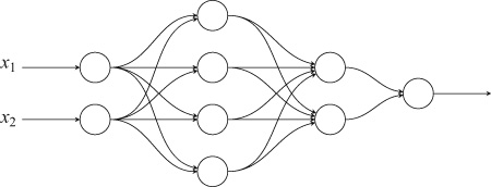
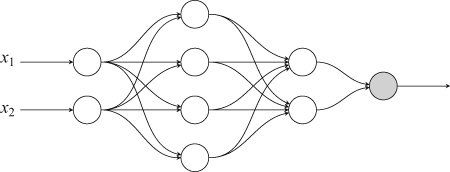
Let us return to a classification task. Our problem now is to pick apart two sets of data, shown in the figure on the top of the next page. The data fall into concentric circles. It is clear to a human that they belong to two distinct groups. It is also clear that they are not linearly separable: no straight line can separate the two classes. We want to create a neural network that will be able to tell the two groups apart so that it will tell us in which group any future observation will belong. This is what you see in the figure at the bottom. For any observation on the light background, the neural network will recognize that it belongs to one group; for any observation on the dark background, it will tell us that it belongs to the other group.
To achieve the results that we see in the lower figure, we build a network layer by layer. We put two neurons on the input layer, one for each coordinate of our data. We add one layer with four neurons, densely connected to the input layer. Because this layer is not connected to the input or output, it is a hidden layer. We add another hidden layer with two neurons, densely connected to the first hidden layer. We finish the network with an output layer of one neuron, densely connected to the last hidden layer. All the neurons use the tanh activation function. The output neuron will produce a value between ![]() and
and ![]() , displaying its belief that the data fall in one or the other group. We’ll take that value and turn it into a binary decision, yes or no, depending on whether it exceeds 0.0 or not. This is what the neural network looks like:
, displaying its belief that the data fall in one or the other group. We’ll take that value and turn it into a binary decision, yes or no, depending on whether it exceeds 0.0 or not. This is what the neural network looks like:


The Backpropagation Algorithm
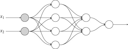
In the beginning, the neural network knows nothing, and no adjustment has taken place; we start with random weights and biases. This is what ignorance means in the neural network world. Then we give the neural network an observation from our data—that is, a set of coordinates. The ![]() and
and ![]() coordinates will go on the input layer. Both neurons take the
coordinates will go on the input layer. Both neurons take the ![]() and
and ![]() values and they pass them as their output to the first hidden layer. All four neurons of that layer calculate their output, which in their turn, they send to the second hidden layer. The neurons on that layer send their own output to the neuron on the output layer, which produces the final output value of the neural network. As the calculations proceed from layer to layer, the neural network propagates the results of the neurons forward, from the input to the output layer:
values and they pass them as their output to the first hidden layer. All four neurons of that layer calculate their output, which in their turn, they send to the second hidden layer. The neurons on that layer send their own output to the neuron on the output layer, which produces the final output value of the neural network. As the calculations proceed from layer to layer, the neural network propagates the results of the neurons forward, from the input to the output layer:


Once we reach the output layer, we calculate the loss, as we did with the single neuron. And then we want to adjust the weights and bias of not just one neuron but rather all the neurons in the network so as to minimize the loss.
It turns out that it is possible to do that by going in the opposite direction, from the output to the input layer. Once we know the loss, we can update the weights and biases of the neurons on the output layer (here we have just a single neuron, but this need is not always so). Having updated the neurons on the output layer, we can update the weights and biases of the neurons on the layer before that—the last hidden layer. Having done that, we can update the weights and biases of the layer before that—the one-but-last hidden layer. And so on, until we reach the input layer:


The way the weights and biases of the neurons are updated is similar to the way a single neuron is updated. Again, the updates are calculated based on mathematical derivatives. You can think of the whole neural network as an enormous function whose variables are the weights and biases of all the neurons. Then we can calculate the derivative of each and every weight and bias with respect to the loss, and use that derivative to update the neuron. With this we arrive at the heart of the learning process in neural networks: the backpropagation algorithm.6
- For each input and desired output,
- 1. Calculate the output and loss of the neural network proceeding layer by layer, going forward from the input to the output layer.
- 2. Update the weights and biases of the neurons to minimize the loss, going backward from the output to the input layer.
Using the backpropagation algorithm, we can build complex neural networks and train them to perform different tasks. The building blocks of deep learning systems are simple. They are artificial neurons, with their limited computational capabilities: taking inputs, multiplying by weights, summing, adding a bias, and applying an activation function on the resulting value. Their power derives from connecting lots and lots of them in special ways, where the resulting networks can be trained to perform the task that we want them to perform.
Recognizing Clothes
To render the discussion more concrete, let us assume that we want to build a neural network that recognizes items of clothing displayed in images, so this is going to be an image recognition task. Neural networks have been found to be exceptionally good at this.
Each image will be a small photo, of dimensions ![]() . Our training data set consists of 60,000 images, and our test data set consists of 10,000 images; we’ll use 60,000 images for training the neural network, and another 10,000 images for evaluating how well it learned. Here is an example image, on which we have added axes and a grid to help the discussion that follows:7
. Our training data set consists of 60,000 images, and our test data set consists of 10,000 images; we’ll use 60,000 images for training the neural network, and another 10,000 images for evaluating how well it learned. Here is an example image, on which we have added axes and a grid to help the discussion that follows:7

The image is broken into small distinct parts because that is how we handle images digitally. Taking the whole image as a rectangular plot, we divide it into small patches, ![]() of them, and each patch is given an integer value from 0 to 255, corresponding to a shade of gray, with 0 being completely white and 255 being completely black. The above image is actually the matrix on the following page.
of them, and each patch is given an integer value from 0 to 255, corresponding to a shade of gray, with 0 being completely white and 255 being completely black. The above image is actually the matrix on the following page.
In reality, neural networks require that we usually scale their inputs to a small range of values, such as between 0 and 1, otherwise they may not work well; you may think of it as having large input values that lead neurons astray. That means that before using this matrix we would divide each cell by 255, but we’ll ignore this in the rest of the discussion.
The different items of clothing may belong to ten different classes, which you can see in the table below. To a computer, the classes are just different numbers, which we call labels:
| Label | Class | Label | Class |
|---|---|---|---|
|
0 |
T-shirt/top |
5 |
Sandal |
|
1 |
Trouser |
6 |
Shirt |
|
2 |
Pullover |
7 |
Sneaker |
|
3 |
Dress |
8 |
Bag |
|
4 |
Coat |
9 |
Ankle boot |

In the following figure, we show a random sample of ten items from each kind of clothing. There is quite a variety in the images, as you can see, and not all of them are picture-perfect examples of each particular clothing class. That makes the problem somewhat more interesting. We want to create a neural network that takes as its input images like these and provides an output that tells us what kind of image it believes its input is.

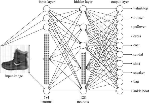
Again, we’ll build our neural network in layers. The first layer, comprising the input neurons, will have 784 neurons. Each one of them will take a single input, from a single patch in the image, and will simply output the value that it gets in its input. If the image is the ankle boot, the first neuron will get the value in the top-left patch, a 0, in its input, and it will output that 0. The rest of the neurons will get the values of the patches proceeding row wise, from top to bottom, left to right. The patch with the value 58, at the right end of the heel of the boot (the fourth row from the bottom, and the third column from the right) will get this 58 and copy it on its output. As rows and columns are counted in the neural network from the top and left, this neuron is in the twenty-fifth row from the top and twenty-sixth column from the left, making it the input neuron number ![]() .
.
The next layer will be densely connected to the input layer. It will consist of 128 ReLU neurons. This layer is not directly connected to the input images (the input layer is) and will not be directly connected to the output (we’ll add another layer for that). Therefore it is a hidden layer, as we cannot observe it from the outside of the neural network. Being densely connected, this will result in a large number of connections between the input and hidden layer. Each neuron on the hidden layer will be connected to the outputs of all neurons on the input layer. There will be 784 input connections per neuron, for a total of ![]() connections.
connections.
We will add another, last layer, which will contain the output neurons that will carry the results of the neural network. This will contain 10 neurons, one for each class. Each output neuron will be connected to all the neurons of the hidden layer, for a total of ![]() connections. The grand total of all the connections between all the layers in the neural network will be
connections. The grand total of all the connections between all the layers in the neural network will be ![]() . The resulting neural work will look, in schematic form, like the one on the next page. As it is impossible to fit all the nodes and edges, you can see dotted boxes standing for the bulk of nodes on the input and hidden layers; there are 780 nodes in the first box and 124 nodes in the second box. We have also collapsed the arrows going to the individual nodes inside the boxes.
. The resulting neural work will look, in schematic form, like the one on the next page. As it is impossible to fit all the nodes and edges, you can see dotted boxes standing for the bulk of nodes on the input and hidden layers; there are 780 nodes in the first box and 124 nodes in the second box. We have also collapsed the arrows going to the individual nodes inside the boxes.
The output of our neural network will consist of 10 outputs, one from each neuron on the layer. Each output neuron will represent one class, and its output will represent the probability that the input image belongs to this class; the sum of the probabilities of all 10 neurons will be 1, as it must happen when we deal with probabilities. This is an example of yet another activation function, called softmax, which takes as input a vector of real numbers and converts them to a probability distribution. Let’s see the two examples that follow.


In the first example, on the left, after training we get this at the output of the network:
| Output Neuron | Class | Probability |
|---|---|---|
|
1 |
T-shirt/top |
0.09 |
|
2 |
Trouser |
0.03 |
|
3 |
Pullover |
0.00 |
|
4 |
Dress |
0.83 |
|
5 |
Coat |
0.00 |
|
6 |
Sandal |
0.00 |
|
7 |
Shirt |
0.04 |
|
8 |
Sneaker |
0.00 |
|
9 |
Bag |
0.01 |
|
10 |
Ankle boot |
0.00 |
That means that the neural network tells us that it is pretty certain it is dealing with a dress, giving it an 83 percent probability, leaving aside small probabilities for the input image being a T-shirt/top, shirt, or trouser.
In the second example, on the right, the network produces:
| Output Neuron | Class | Output |
|---|---|---|
|
1 |
T-shirt/top |
0.00 |
|
2 |
Trouser |
0.00 |
|
3 |
Pullover |
0.33 |
|
4 |
Dress |
0.00 |
|
5 |
Coat |
0.24 |
|
6 |
Sandal |
0.00 |
|
7 |
Shirt |
0.43 |
|
8 |
Sneaker |
0.00 |
|
9 |
Bag |
0.00 |
|
10 |
Ankle boot |
0.00 |
The neural network is 43 percent certain that it is dealing with a shirt—and it is wrong; the photo is really a picture of a pullover (in case you couldn’t tell). Still, it did give its second best, at 33 percent, to the image being a pullover.
We gave one example where the network comes up with the right answer, and another instance where the network comes up with the wrong answer. Overall, if we give the network many images to recognize, all the 60,000 images in our training data set, we’ll find out that it manages to get right about 86 percent of the 10,000 images in the test data set. That is not bad, considering that the neural network, even though it is way more complicated than the previous one, is still a simple one. From this baseline, we can create more complicated network structures that would give us better results.
Despite the increased complexity, our neural network learns in the same way as our simpler networks recognizing blobs of data and concentric circles. For each input during training we obtain an output, which we compare to the desired output to calculate the loss. The output now is not a single value but rather 10 values, yet the principle is the same. When the neural network recognizes a shirt with about 83 percent probability, we can compare that with the ideal, which would be to recognize it with 100 percent probability. Therefore we have two sets of output values: the one obtained by the network, with various probabilities assigned to the different kinds of clothes, and what we would like to have gotten from the network, which is a set of probabilities where all of them are zero apart from a single probability, corresponding to the right answer, which is equal to one. In the last example, the output contrasted to the target would be as follows:
| Output Neuron | Class | Output | Target |
|---|---|---|---|
|
1 |
T-shirt/top |
0.00 |
0.00 |
|
2 |
Trouser |
0.00 |
0.00 |
|
3 |
Pullover |
0.33 |
1.00 |
|
4 |
Dress |
0.00 |
0.00 |
|
5 |
Coat |
0.24 |
0.00 |
|
6 |
Sandal |
0.00 |
0.00 |
|
7 |
Shirt |
0.43 |
0.00 |
|
8 |
Sneaker |
0.00 |
0.00 |
|
9 |
Bag |
0.00 |
0.00 |
|
10 |
Ankle boot |
0.00 |
0.00 |
We take the last two columns and we calculate again a loss metric—only this time, as we do not have a single value, we do not calculate a simple squared difference. There exist metrics to calculate the difference between sets of values like these. In our neural network we used one such metric, called categorical cross-entropy, which indicates how much two probability distributions differ. Having calculated the loss, we update the neurons on the output layer. Having updated them, we update the neurons on the hidden layer. In short, we perform backpropagation.
We go through the same process for all images in our training data set—that is, for a whole epoch. When we are done, we do this all over again for another epoch. We repeat the process while trying to strike a balance: enough epochs so that the neural network will learn as much as possible from the training data set without going into too many epochs where the neural network will learn too much from the training data set. During learning, the network will be adjusting the weights and biases of its neurons, which are a lot. The input layer just copies values to the hidden layer, so no adjustments need to be done to the input neurons, but there are 100,352 weights on the hidden layer, 1,280 weights on the output layer, 128 biases on the hidden layer, and 10 biases on the output layer, for a total of 101,770 parameters.
Getting to Deep Learning
It can be proven that even though a neuron on its own cannot do much, a neural network can perform any computational task that can be described algorithmically and run on a computer. Therefore there is nothing that a computer can do that a neural network could not do. The whole idea, of course, is that we do not need to tell the neural network exactly how to perform a task. We only need to feed it with examples while using an algorithm to make the neural network learn how to perform the task. We saw that backpropagation is such an algorithm. Although we limited our examples to classification, neural networks can be applied to all sorts of different tasks. They can predict the values of a target quantity (for instance, credit scoring), translate between languages as well as understand and generate speech; and beat human champions in the game of Go, in the process baffling experts by demonstrating completely new strategies of playing a centuries-old game. They have even learned how to play the game of Go starting with just a knowledge of the rules, without access to a library of previously played games, and then proceeding to learn as if the neural network were playing games against itself.8
Today, successful applications of neural networks abound, yet the principles are not new. The Perceptron was invented in the 1950s, and the backpropagation algorithm is more than 30 years old. In this period, neural networks came and went out of fashion, with enthusiasm for their potential ebbing and flowing. What has really changed in the last few years is our capability to build really big neural networks. This has been achieved thanks to the advances in manufacturing specialized computer chips that can perform the calculations executed by neurons efficiently. If you picture all the neurons of a neural network arranged inside a computer’s memory, then all the required computations can be carried out by operations on vast matrices of numbers. A neuron calculates the sums of the weighted products of its inputs; if you recall the discussion on PageRank in the previous chapter, the sum of the products is the essence of matrix multiplication.
It has turned out that graphics processing units (GPUs) are perfectly suited for this. GPUs are computer chips that are specially designed to create and manipulate images inside a computer; the term builds on central processing units (CPUs), the chip that carries out the instructions of a program inside a computer. GPUs are built to carry out instructions for computer graphics. The generation and processing of computer graphics requires numerical operations on big matrices; a computer-generated scene is a big matrix of numbers (think of the shoe). GPUs are the workhorses of game consoles. The same technology that arrests human intelligence in hours of diversion is also used to advance machine intelligence.
We started with the simplest possible neural network, consisting of a single neuron. Then we added a few neurons, and then we added a few more hundreds. Still, the image recognition neural network that we created is by no means a big one. Nor is its architecture complicated. We just added layer on layer of neurons. Researchers in the field of deep learning have made big strides in devising neural network designs. These architectures may comprise dozens of layers. The geometry of these layers need not be a simple one-dimensional set of neurons, like the ones we have here. For example, neurons inside a layer may be stacked on two-dimensional canvas-like structures. Moreover, it is not necessary to have each layer densely connected to the one before; other connection patterns are possible. Nor is it necessary to have the outputs of a layer simply connected to the inputs of the next layer. We may, for instance, have connections between non-consecutive layers. We may bundle up layers and treat them as modules, combining them with modules containing other layers to form more and more complex configurations. Today we have a menagerie of neural network architectures at our disposal, such that particular architectures are well suited for specific tasks.
The neurons on the layers in all the neural network architectures update the values of the weights and biases as they learn. If we reflect on what is happening, we can see that we have a set of inputs that transforms the layers during the learning process. Once the training stops, the layers have somehow, via the adjustments in their parameters, taken in the information represented by the input data. The weights and biases configuration of a layer represents the input it has received. The first hidden layer, which comes in direct contact with the input layer, encodes the neural network’s input. The second hidden layer encodes the output of the first hidden layer, to which it is directly connected. As we proceed deeper and deeper into a multilayer network, each layer encodes the output received by the previous layer. Each representation builds on the previous one and therefore is on a higher level of abstraction from the one of the preceding layer. Deep neural networks, then, learn a hierarchy of concepts, proceeding to higher and higher levels of abstraction. It is in this sense that we talk of deep learning. We mean an architecture whereby successive levels represent deeper concepts, corresponding to higher levels of abstraction. In image recognition, the first layer of a multilayer network may learn to recognize small local patterns, such as edges in the image. Then the second layer may learn to recognize patterns that are built from the patterns recognized by the first layer, such as eyes, noses, and ears. The third layer may learn to recognize patterns that are built from the patterns recognized by the second layer, like faces. Now you can see that our neural network for recognizing the images was somewhat naive; we did not try to implement actual deep learning. By building abstractions on abstractions, we expect our network to find patterns that humans find, from structures in sentences, to signs of malignancy in medical images, to recognizing handwritten characters, to detecting online fraud.
Yet, you may say, it all boils down to updating simple values on simple building blocks—the artificial neurons. And you would be correct. When people realize that, sometimes they feel let down. They want to learn what machine and deep learning are, and the simplicity of the answer disappoints: something that appears to have human capabilities can be reduced to fundamentally elementary operations. Perhaps we would prefer to find something more involved, which would not fail to flatter our self-esteem.
We should not forget, however, that in science we believe that nature can be explained from first principles, and try to find such principles that are as simple as possible. That does not preclude complex structures and behaviors arising out of simple rules and building blocks. Artificial neurons are much simpler than biological ones, and even if the workings of biological neurons can be explained in simple models, it is thanks to the vast number of interconnected biological neurons that intelligence, as we know it, can arise.
This helps put some things into perspective. True, artificial neural networks can be uncanny in their potential. In order to make them work, however, an amazing amount of human creativity and terrific engineering effort is required. We have only scratched the surface in our account here. For instance, take backpropagation. That is the fundamental algorithm behind neural networks, allowing us to perform efficiently what is at heart a process of finding mathematical derivatives. Researchers have been busy devising efficient calculation techniques, such as automatic differentiation, a mechanism for calculating derivatives that has been widely adopted. Or take the exact way that changes in the neural network parameters are calculated. Various different optimizers have been developed, allowing us to deploy bigger and bigger networks that are at the same time more and more efficient. Turning to the underlying hardware, hardware engineers are designing better and better chips to run more and more neural computations faster while using less computing power. Looking at network architectures, new neural network architectures are proposed that improve on existing ones. This is a hotbed of research and experimentation, and even encompasses efforts to build neural networks that design other neural networks. So every time you see a news report that a neural network has reached a new achievement, doff your hat to the hardworking people who made this possible.9
Artificial neurons are much simpler than biological ones, and even if the workings of biological neurons can be explained . . . , it is thanks to the vast number of interconnected biological neurons that intelligence . . . can arise.