In this appendix, I review the basic Microsoft Excel skills that you may need to get the most benefit from some chapters in this book. If you plan to download and work with the sample workbooks from my website, www.stephenlnelson.com, you need some of the skills that this primer covers.
If you’ve used Excel much — even for just a few weeks — you probably possess all these skills. Nevertheless, if you’re even a teensy bit concerned about whether you have the right skills, take the time to read this appendix.
Note: I used Excel 2016 and Windows 10 when writing this appendix. If you’re using an earlier or later version of Excel, you may notice some slight differences between the images that appear here and what you see on your monitor. If you need detailed guidance, pick up Excel 2016 For Dummies, by Greg Harvey (John Wiley & Sons, Inc.).
Starting Excel
You can start Excel in two ways, neither of which requires a PhD in physics. You can click the Start button and then click the Excel tile that appears on the Start menu’s list of programs, or you can open an Excel workbook.
If you’re going to use the Excel tile, you simply find the Excel tile (you may need to scroll around the Start menu’s list of tiles) and then click it.
To start Excel by opening an Excel workbook, you select the workbook from a menu or in a folder window. You commonly see documents, including Excel workbooks, listed on menus — both Windows menus and Program menus. If Windows displays the list of documents in a folder window, for example (see Figure A-1), you can open the workbook by double-clicking it. When you open an Excel workbook, Windows starts Excel and tells it to open the workbook.
FIGURE A-1: A folder that shows an Excel workbook.
Stopping Excel
To stop Excel, click the Excel window’s Close box. When you stop Excel, Excel closes any of the open Excel workbooks before it stops.
The Close box is the button marked with an X that appears in the top-right corner of the Excel window.
Explaining Excel’s Workbooks
After you start Excel, it displays an empty workbook with one worksheet in its document window. Figure A-2 shows a picture of an empty workbook.
FIGURE A-2: The Excel window with an empty workbook.
An Excel workbook is just a spreadsheet. A spreadsheet is comprised of numbered rows and lettered columns. You see the row numbers along the left edge of the spreadsheet, and you see the lettered columns along the top edge of the spreadsheet. The first row is numbered 1, the second is numbered 2, and so on. The first column is labeled with the letter A, the second column is labeled with the letter B, and so on.
The intersections of rows and columns are called cells. A cell location is described by using the column letter and row number. The cell in the top-left corner of the workbook, for example, is labeled A1.
Putting Text, Numbers, and Formulas in Cells
You build a workbook, or spreadsheet, by entering text labels, numbers, and formulas in the cells that comprise a workbook. The following list details these items:
Text labels include letters and numbers that you don’t want to use in calculations. Your name, some budget expense description, and a telephone number are examples of text labels. None of these pieces of information is used in calculations.
Numbers, or values, are bits of data that you may want to use later in a calculation. The actual amount that you budgeted for some expense, for example, will always be a number or value.
Formulas are also entered into worksheet cells. If you enter =2+2 into a cell, Excel doesn’t display the formula. Rather, it calculates the formula result and displays that. The formula is what is actually stored in the cell, but the formula result is displayed.
This business about formulas going into workbook cells is, essentially, the heart of Excel. Even if an Excel workbook did nothing else, it would still be an extremely valuable tool. In fact, the first spreadsheet programs did little more than calculate cell formulas.
To enter a text label, a value, or a formula into a cell, all you do is click the cell by using the mouse and then type the text label, value, or formula. When you press Enter or click another cell, Excel enters your label, value, or formula into the cell. That’s all it takes.
Writing Formulas
In the preceding section, I tell you about formulas and even show you a simple formula example. But to use formulas practically, you need to possess several other pieces of knowledge. Specifically, you need to remember several things about entering formulas into the cells of a workbook:
Formulas should begin with the equal sign (=). The equal sign tells Excel that what follows is a formula that it should calculate.
You can use any of the standard arithmetic operators in your formulas. To add numbers, use the addition sign (+). To subtract numbers, use the subtraction operator (–). To multiply numbers, use the multiplication operator (*). To divide numbers, use the division operator (/). You can also perform exponential operations by using the exponential operator (^).
You aren’t limited to using values in your formulas. You can also use cell addresses. When you use a cell address in a formula, Excel uses the value or formula result from that cell in the calculation. If cell A1 holds the value 2, and cell B1 holds the value 2, the formula =A1+B1 returns the value 4. In other words, this formula is equivalent to =2+2.
Remember standard rules of operator precedence when you build complicated formulas. As you may remember from junior-high math, exponential operations are performed first. Multiplication and division operations are performed second. Addition and subtraction operations are performed third. To override these standard rules of operator precedence, you place the operations that you want performed first inside parentheses. Table A-1 shows some example formulas and the formula results to illustrate these rules of precedence. If you get the rules wrong, you’ll have to stay after class.
The cells that you see inside the Excel program window represent only a small portion of the Excel workbook. An Excel workbook actually provides more: 1,048,576 rows and, oh, about 16,000 columns.
Because the alphabet provides only 26 letters, a new naming scheme is needed, starting in column 27. Excel labels the 27th and subsequent columns by using two letters. The 27th column is labeled AA, the 28th column is labeled AB, and the 29th is labeled AC. This scheme goes all the way through the 702nd column, which is labeled ZZ.
Taking it up a notch, Excel labels the 703rd and subsequent columns by using three letters. The 703rd column is labeled AAA, the 704th column is labeled AAB, the 705th column is labeled AAC, and so on. The last, or rightmost, column in an Excel workbook is labeled XFD.
You can scroll the viewable portion of the Excel worksheet in several ways:
Use the horizontal and vertical scroll bars that appear along the bottom edge and at the right edge of the worksheet window. You can click the scroll bar, drag the scroll marker, and click the scroll-bar arrow buttons that appear at either end of the scroll bar. If you’re not familiar with how scroll bars work, take the time to experiment and see what they do.
Scroll the viewable portion of the Excel worksheet by moving the cell selector. The cell selector is the dark rectangular border that Excel uses to mark the active cell. The active cell is the cell in which whatever you type gets placed. You can move the cell selector by pressing the arrow keys; Excel moves the cell selector in the direction of the arrow. If you aren’t sure what the cell selector is, press the arrow keys a bunch of times. See that rectangle that jumps around? That’s the cell selector.
Move the viewable portion of the worksheet up and down by pressing the Page Up and Page Down keys. Just try this, okay, if you need more help to see what I mean. Press the Page Down key a few times. Press the Page Up key a few times. Now you’ve got it.
You have several other ways to scroll within a worksheet. If you’re really interested, you may want to look up the other scrolling methods in Excel’s online Help or get a good book like a recent edition of Excel For Dummies, by Greg Harvey (Wiley).
Copying and Cutting Cell Contents
You can easily copy and paste contents of worksheet cells, and you want to do both of these things because worksheet construction becomes much easier when you use these skills.
Copying cell contents
To copy cell contents, follow these steps:
Select the cells that you want to copy.
To select a single cell, click that cell. To select a range of cells — a range is just a group of contiguous cells — click the cell in the top-left corner and then drag the mouse to the cell in the bottom-right corner of the range.
Copy the selection by clicking the Copy icon.
First, if necessary, click the Home tab on the Ribbon to display the Home icons. (You may need to do this because the Copy icon, which you use for copying, appears on the Home tab.) Excel places a copy of the contents of the selection on the Office Clipboard, which is a temporary storage area.
Note: The Copy icon looks like two miniature duplicated documents.
Select the location where you want to place the copied data.
To tell Excel where you want to put the selection, click the cell in the top-left corner of the range into which you want to copy the data.
Paste the copied range selection by clicking the Paste icon.
Excel copies the previously copied range selection from the Office Clipboard to the workbook location that you identify in Step 3.
Note: The Paste icon looks like a clipboard with a piece of paper attached.
Moving cell contents
You can move, or cut, the contents of cells and ranges by following these steps:
Select the cells that you want to move.
To select a single cell, click that cell. To select a range of cells, click the cell in the top-left corner and then drag the mouse to the cell in the bottom-right corner.
Choose the Cut command.
You tell Excel that you want to cut your selection by clicking the Cut icon that appears on the Home tab on the Ribbon. When you choose the Cut command, Excel moves the contents of the selection to the Office Clipboard. Again, if you can’t see the Cut icon, click the Home tab on the Ribbon to display the Home icons.
Note: The Cut icon looks like a pair of scissors.
Select the location where you want to place the data you’re moving.
To tell Excel where to move the selection, click the cell in the top-left corner of the range into which you want to move the data.
Paste the data by choosing the Paste command.
Alternatively, you can click the Paste toolbar button. When you do, Excel copies the previously copied range selection from the Office Clipboard to the workbook location that you identify in Step 3.
Moving and copying formulas
You can move and copy formulas the same way that you move and copy other stuff stored in cells. You need to know something really important about copying formulas, however: Excel adjusts the cell addresses used in a formula when you copy the cell or cells that store the formula.
This sounds very strange, but let me show you a quick example of how this adjustment occurs. You’ll see immediately why the adjustment is useful. Take a look at the simple budgeting workbook shown in Figure A-3. As you can see, this simple spreadsheet calculates totals for a budget. The totals appear in row 6. Because Excel adjusts cell addresses when it copies them, if you copy the formula in cell B6 to cells C6 and D6, Excel ends up placing the correct formula in cells C6 and D6.
FIGURE A-3: A simple worksheet that budgets expenses.
In cell B6, the formula is =B2+B3+B4+B5. This formula sums the values for the first month. Obviously, however, you don’t want to use this formula in cell C6. Excel guesses that this is the case when it copies the formula from B6. What Excel places in cell C6, therefore, is the formula =C2+C3+C4+C5. What Excel places in cell D6 is the formula =D2+D3+D4+D5.
Excel doesn’t adjust the cell addresses in formulas in a range selection when you move cell contents. The adjustment of cell addresses and formulas occurs only when you copy formulas.
You can flag, or mark, those cell addresses that you don’t want adjusted when they’re copied. To do this, you precede the column letter and row number with a dollar sign ($) to tell Excel that the address shouldn’t be adjusted. If the cell address $A$1 is used in a formula, for example, Excel won’t adjust the column letter or row number if it copies the formula. Excel calls these fixed cell addresses absolute references. You can also tell Excel to adjust only one portion of the cell address by using the dollar sign ($) in front of only the column letter or the row number. If the cell address A$1 is used in a formula, Excel adjusts the column letter but not the row number.
Formatting Cell Contents
Excel allows you to format the contents of the cells in a worksheet. You can choose the font, the point size, and special effects such as boldfacing, underlining, or italicizing for a workbook or a range.
For values and formula results, you can also add standard punctuation, including dollar signs, percentage symbols, decimal points, and commas for separating thousands.
In general, you format a cell or range by selecting the range and then using the Home tab’s formatting boxes and buttons or by opening the Format Cells dialog box, which you do by pressing Ctrl+1 (the number 1).
When you point to an icon, button, or box, Excel displays the item’s name in a box next to the item. A bit of poking around, then, quickly lets you figure out which boxes and buttons are which.
The Home tab on the Ribbon, for example, provides a font box that you can use to select the font for the selected range. The Home tab also provides a Font Size box for specifying the point size of text and numbers in the selected range.
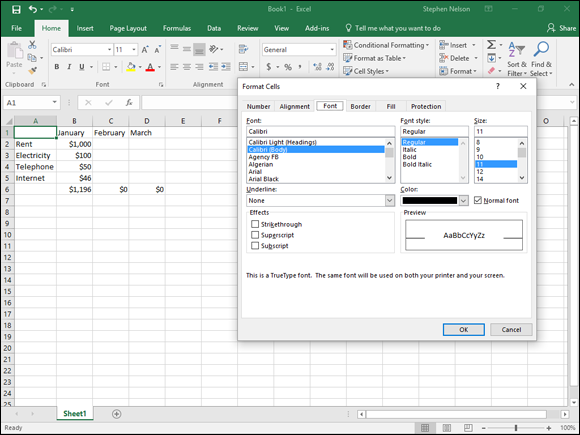
The Format Cells dialog box provides tabs of boxes and buttons for formatting the contents of cells. If you want to change the font used in a range selection, click the Format Cells: Font icon and then use the Font tab’s boxes and buttons to make your changes. The Format Cells: Font icon is the little arrow in the bottom-right corner of the Font section on the Ribbon’s Home tab. Figure A-4 shows the Font tab of the Format Cells dialog box.
FIGURE A-4: The Font tab of the Format Cells dialog box.
Recognizing That Functions Are Simply Formulas
Here’s another important tidbit to know about Excel: Although you can construct very complicated formulas by using the standard arithmetic operators, Excel provides prefabricated formulas called functions that make it easy to calculate standard measurements. Excel provides a function to easily calculate an arithmetic mean, or average, for example. It also provides a function to calculate the payment on a car loan.
A simple example demonstrates how this works. If you look back at the worksheet shown in Figure A-3, you can see (or guess) that the formula in cell B6 adds the values in B2, B3, B4, and B5. With what you already know about Excel formulas, you can construct a total formula that adds these values. You can enter the formula =B2+B3+B4+B5 into cell B6.
If you look closely at the area that’s just below the Excel Ribbon (Microsoft’s name for Excel’s menu), you can see what’s known as the formula bar. The formula bar shows you the contents of the selected cell. In Figure A-3, the selected cell is B6, so the formula bar shows you the contents of cell B6, which happens to be the formula that adds the values in cells B2, B3, B4, and B5.
You can also use a function to make this calculation. To add a series of values, you use the SUM function. Then you include as function arguments, or function inputs, the individual values, individual cell addresses, or range selections. To see how this works in the case of the worksheet shown in Figure A-5, you can enter the formula =SUM(B2:B5) into cell B6.
Function formulas use a standard set of conventions:
The first part of this formula is the equal sign (=). Because functions are formulas, you begin a function with an equal sign.
The next part of the function formula gives the function name. In the case of the SUM function, the function name is SUM.
The third part of the formula function includes the function inputs, or arguments, inside parentheses. In the worksheet shown in Figure A-5, the inputs are included as a range reference (B2:B5).
Sometimes, functions are so simple that you won’t need any help remembering how the arguments should appear or what arguments the function needs. The SUM function, for example, is one that spreadsheet users construct so frequently that they usually memorize its syntax after only a few uses.
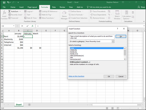
Other functions, however, such as the functions to calculate a loan payment, require several arguments in a particular order. For more complicated functions, you typically want to use the Insert Function command. To use the Insert Function command, click the Formulas tab and then click the Insert Function icon. (The icon shows a little fx label and is located just to the left of the formula bar.) Excel displays the Insert Function dialog box, as shown in Figure A-6.
If you don’t know what function you want, you can type a brief description of whatever you want to calculate in the Search for a Function text box, shown at the top of the dialog box, and click Go. Alternatively, you can select a category of functions from the Or Select a Category drop-down list. This list provides several categories of functions, including financial functions, date and time functions, mathematical and trigonometric functions, statistical functions, and text functions.
Based on what you type in the first text box or based on the category that you select from the drop-down list, Excel displays a list of possible functions in the bottom portion of the Insert Function dialog box. You search this list for the function that you want. If you select a function in the list, Excel displays a brief description of the function and shows the arguments needed for the function to calculate.
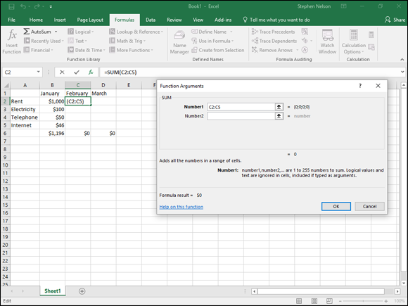
After you find and select the function that you want to use, click OK. Excel displays the Function Arguments dialog box, as shown in Figure A-7. The Function Arguments dialog box provides text boxes that you use to supply the arguments, or inputs, to the function. Function arguments can be values or cell addresses.
After you supply the needed function arguments, click OK. Excel enters a formula function into the active cell by using the function name and function arguments that you provided.
As I mention earlier, after you know a function’s arguments, you can type the function directly in cells. To do this, click the cell; then type the equal sign, the function name, and then the beginning parenthesis [(]. Excel displays a pop-up box that names the arguments (just to remind you of their order). You enter each of the arguments, separating individual arguments with commas. After you type the last argument, type the ending parenthesis [)] and then press Enter.
Saving and Opening Workbooks
As you may expect if you’ve worked with other Microsoft Office applications, such as Microsoft Word, Excel saves and opens its workbook documents in a predictable way.
Saving a workbook
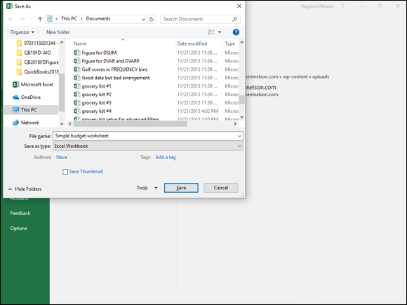
To save a workbook, choose File ⇒ Save. The first time that you want to save a workbook, you choose either File ⇒ Save or File ⇒ Save As. In either case, Excel displays the Save As window (not shown), which asks where you want to save your workbook, and you pick the storage location you want to use. If you click More Options, Excel displays the traditional Save As dialog box, shown in Figure A-8.
You enter a name for the workbook by using the File Name box. Typically, you don’t have to worry about any of the other buttons or boxes on the Save As dialog box. You simply click the Save button. Excel saves your workbook in a specified location by using the specified name.
After you save a workbook for the first time, you can save the workbook again simply by choosing File ⇒ Save again. When you do, Excel saves the workbook, using the same name and the same location.
If you want to save a copy of the workbook in a new location or use a new name, you choose File ⇒ Save As. Excel displays some recent folders you may have used, so click the folder you want to save it to, if you see it. If you don’t see the folder, click More Options to see the traditional Save As dialog box (refer to Figure A-8) to select a certain location. Just as you do the first time you save a workbook, you choose a storage location for the workbook in the Save As window and then provide a name for the workbook in the File Name text box.
Opening a workbook
To open an existing workbook, you can either display the contents of the folder storing the workbook or open Excel and then choose File ⇒ Open.
If you want to open Excel workbook documents directly from Windows, first display the folder’s window. When Windows shows the Excel workbook document that you want to open in a folder window, simply double-click the workbook. Windows starts Excel and tells it to open the workbook.
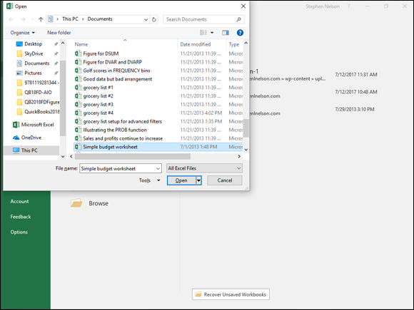
You can also open workbook documents by choosing File ⇒ Open. When you do, Excel first displays the Open window, which you use to identify the storage location of the workbook (such as your computer) by clicking the location. After you identify the storage location, Excel displays the Open dialog box, as shown in Figure A-9. To use the Open dialog box, select the workbook that you want to open from the list Excel displays and then click Open.
You print Excel workbooks in roughly the same manner that you print other documents. First, you start Excel and open the document — in the case of Excel, a workbook — that you want to print.
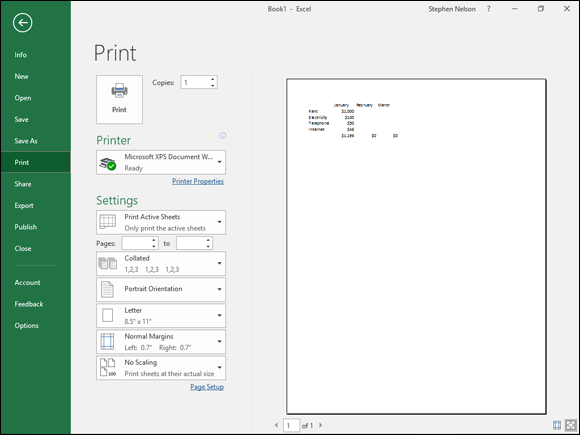
After Excel opens the workbook, choose File ⇒ Print. Excel displays the Print dialog box, shown in Figure A-10, which shows you how the printed workbook will look and contains buttons and boxes that you use to control printing. Use the Copies box to specify how many copies of the workbook you want to print. Select the printer you want to use from the Printer drop-down list. Use the Settings buttons and drop-down lists to specify what part of the workbook you want to print. Then click Print.
If you have a question about one of the buttons or boxes in the Print dialog box, click the question mark (?) button, located in the top-right corner of the dialog box, and then click the button or box that you don’t understand. A text box offering context-sensitive help appears.
Often, you’ll have a workbook that looks perfect onscreen (and is), only to realize that it was just a little bit too wide to fit on a single sheet of paper. When this happens, Excel prints two pages for every page that you think you’re printing, thus leaving you to reprint — or tape all those sheets together in a haphazard banner. A quick preview would save you all this grief (not to mention time, ink, and paper).
One Other Thing to Know
The preceding lists of skills don’t cover every feature or function of Excel. With the skills that I’ve just described, however, you can do most of the things that people do with Excel.
If you’ve been working with other Windows applications — particularly Microsoft Office applications — you can see that none of what you’re going to do with Excel is all that complicated. Mostly, it comes down to entering text labels, values, and simple formulas into worksheet cells. And although your formulas may become very complicated, the mechanics of using Excel to build those formulas aren’t particularly difficult.
If you’ve read the preceding paragraphs of this appendix and find yourself scratching your head, you probably need to find out more about Excel from some other resource. You may be able to get the skills that you need simply by experimenting with Excel. You may also want to pick up a good tutorial on Excel, such as a recent edition of Excel For Dummies, by Greg Harvey (Wiley).

 The Close box is the button marked with an X that appears in the top-right corner of the Excel window.
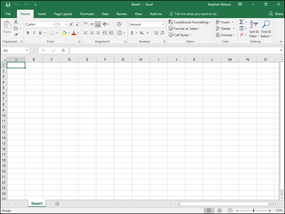

 Excel doesn’t adjust the cell addresses in formulas in a range selection when you move cell contents. The adjustment of cell addresses and formulas occurs only when you copy formulas.