Chapter 4
Modeling the Existing Terrain Using Surfaces

In Chapter 3, “Establishing Existing Conditions Using Survey Data,” you learned how to establish the existing conditions of a project by playing a very elaborate game of connect-the-dots. So far, you’ve been solving the connect-the-dots puzzle in only two dimensions—creating the treelines, fence lines, buildings, trees, and so on. Now, you’ll use the same data to establish the third dimension of your existing conditions model, and you’ll do that using AutoCAD^® Civil 3D^®surfaces.

Many would say the goal in this process is to generate existing contours for the project. Twenty years ago, that would have been the case; but in this era of 3D modeling, the result of your efforts will serve a much greater purpose. Although it’s true that you’ll be able to create contours from your surface model, you’ll also create an accurate 3D representation of the ground that can be used in many ways throughout the project.

In this chapter, you’ll learn to

Understand the purpose and function of surfaces
Create a surface from survey data
Use breaklines to improve surface accuracy
Edit surfaces
Display and analyze surfaces
Annotate surfaces

Understanding Surfaces

As you might guess, the 3D game of connect-the-dots is a bit more sophisticated than the 2D version. In addition, you need the result to be a 3D model rather than just lines. To accomplish this, Civil 3D uses a computer algorithm that connects the dots in the most efficient and accurate way possible. This algorithm is known as a Triangular Irregular Network (TIN).

The TIN algorithm works by connecting one point to at least two of its neighbors using 3D lines. Because each point connects to two or more of its neighbors, the resulting model looks something like a spider web made up of triangles (the T in TIN). Because the spacing between points is typically nonuniform, the triangles come in many shapes and sizes, which is why it’s called irregular (the I in TIN). The network (the N in TIN) part comes from all the points being connected by lines, and the points and lines being related to one another. Figure 4-1 shows a surface with its TIN lines visible.

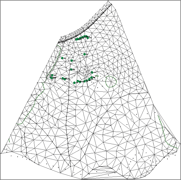
c04f001.tif — **Figure 4-1:** A surface model displayed as TIN lines. Note the irregular triangular shapes that make up the surface model.

There’s even more to it than the triangles, though. In fact, the triangles are just a handy visual representation of the algorithm at work, and, by themselves, they aren’t all that useful. What is useful is that the algorithm can calculate the elevation of any point within the area covered by the TIN model. So, even if you pick a point in the open space inside a triangle, the elevation will be calculated. This is what makes the TIN model a true model. It can be sliced, be turned on its side, have water poured on it, be excavated, and be filled in—all virtually, of course. The capability of using surface models for these types of calculations and simulations is what makes them so useful and puts them at the core of Civil 3D functionality.

Creating a Surface from Survey Data

You create a surface in Prospector by simply right-clicking the Surfaces node of the tree and selecting Create Surface, as shown in Figure 4-2. The newly created surface appears in Prospector immediately, but it can’t be seen in the drawing until some data is added to it. The fundamental components of a surface are points and lines. It’s your job to supply the source of the points, and Civil 3D takes care of drawing the lines. At this phase of the project, you’ll be using survey points as the initial source of surface-point data.

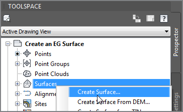
c04f002.tif — **Figure 4-2:** Creating a surface from within Prospector

Exercise 4.1: Create an Existing Ground Surface

In this exercise, you’ll create a surface from survey data.

If you haven’t already done so, go to the book’s web page at www.sybex.com/go/civil3d2015essentials and download the files for Chapter 4. Unzip the files to the correct location on your hard drive according to the instructions in the introduction. Then, follow these steps:

Open the drawing named Create an EG Surface.dwg located in the Chapter 04 class data folder.
In Prospector, right-click Surfaces and select Create Surface.
In the Create Surface dialog box, enter EG in the Name field.

EG stands for existing ground.
For Style, select C-Existing Contours (1') (C-Existing Contours (0.5m)). Click OK to dismiss the Create Surface dialog box.
In Prospector, expand Surfaces ⇒ EG ⇒ Definition. Study the items listed beneath EG in the tree (see Figure 4-3).

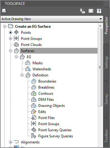
Figure 4-3: The contents of a surface shown in Prospector
Right-click Point Groups, and select Add.
Select Ground Shots, and click OK. The surface is now visible in plan view in the form of contours and shaded 3D faces in the bottom-right 3D view.

The difference in appearance between plan view and 3D view is a function of the surface style.
In the lower-right viewport, click Shaded and select 2D Wireframe, as shown in Figure 4-4. The appearance of the surface changes to show the TIN lines.

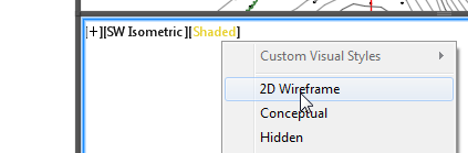
Figure 4-4: Changing the visual style to 2D Wireframe in the lower-right viewport
Click 2D Wireframe and select Conceptual. To orbit your view of the surface, click and drag center mouse button while holding your Shift key. Observe the surface from several different viewpoints.

This way of studying the surface gives a real sense of the surface as a “solid” model in which the area inside the triangles has substance. It’s also a great visual representation of the TIN algorithm and the surface model (see Figure 4-5).
Save and close the drawing.
You can view the results of successfully completing this exercise by opening Create an EG Surface - Complete.dwg.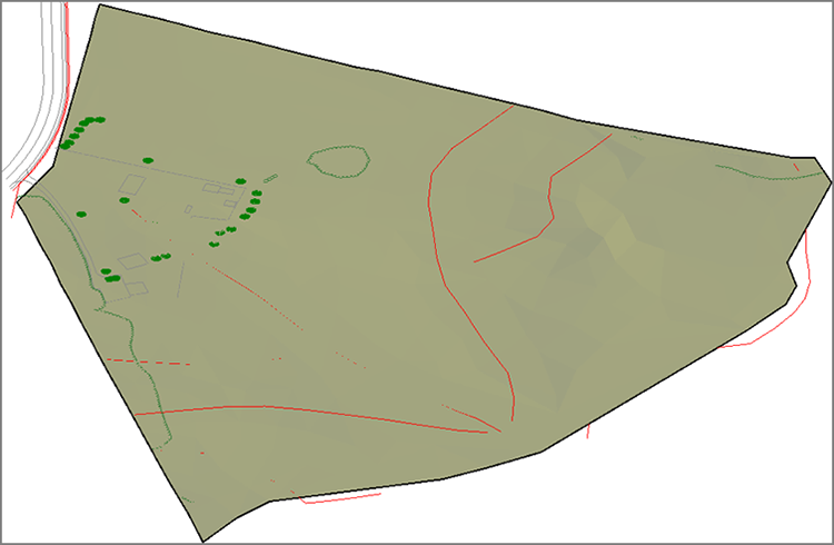

Figure 4-5: A surface shown using the Conceptual visual style

Using Breaklines to Improve Surface Accuracy

The TIN algorithm creates surfaces by drawing 3D lines between points that are closest to each other. In certain instances, this is not the most accurate way to model the surface, and the TIN lines must be forced into a specific arrangement. This arrangement typically coincides with a linear feature such as a curb, the top of an embankment, or a wall. This forced alignment of TIN lines along a linear feature is best handled with a breakline. In Figure 4-6, the blue lines represent the edges of a channel and the TIN lines are shown in red. In the image on the top, the blue lines have not been added to the channel surface as breaklines, resulting in a rough and inaccurate representation of the channel. In the image on the bottom, the breaklines have been applied and force the TIN lines to align with the edges of the channel, producing a much smoother and more accurate model.

From Prospector, you can add breaklines by right-clicking the Breaklines node for a given surface and selecting Add (see Figure 4-7). When it comes to survey data, there is an even easier way. From the Survey Toolspace, you can right-click Figures and select Create Breaklines. This opens a list of all your survey figures with some checked as breaklines and some not (see Figure 4-8). How does the command know which is which? This was specified in the figure prefix database you learned about in Chapter 3. As the figures were created, they were automatically tagged as breaklines or non-breaklines according to the code assigned to the points that define them.

Components of a Surface

As shown in Figure 4-3, you can use many potential types of information to create a surface and control its shape. The following list describes each one briefly:

Boundaries Boundaries are used to control where the surface is. A boundary around the edge of a surface can keep it contained within a certain area. Another type of boundary can keep a surface out of an interior area, like a pond or building.
Breaklines Breaklines force TIN lines to align with them. In this way, they help to define hard edges such as edges of embankments, curb lines, ditch lines, and so on.
Contours Usually, we think of contours as the end product of building a surface, but they can also be used as a source of data for a surface.
DEM Files DEM stands for digital elevation model, and it’s typically associated with large-scale mapping that has relatively low accuracy. DEMs can often be found alongside large-scale mapping data and are typically only accurate enough for rough analysis or calculations.
Drawing Objects Drawing objects are AutoCAD^® software entities such as lines, blocks, and even text. These items can be used to help define a surface as effectively as survey points, as long as they’ve been created at the appropriate elevations.
Edits Edits aren’t actual data, but they do contribute to the makeup of a surface. There are many ways in which a surface can be edited to improve its accuracy or usability. Some of these editing methods will be covered in this chapter.
Point Files You’ve already learned that a point file is a text file containing x, y, and z data. So far, you’ve used these files to create Civil 3D points in the drawing, but the same data can also be imported directly into a surface.
Point Groups In Chapter 3, you learned that one of the benefits of point groups is that they enable multiple points to be selected simultaneously. Using one or more point groups to define a surface is one of the most important and most common uses of point groups in Civil 3D.
Point Survey and Figure Survey Queries These queries are created using the survey functionality and utilize a sophisticated way of selecting points and figures based on survey properties. These queries are not covered in this book but information about them is available within the Civil 3D help.

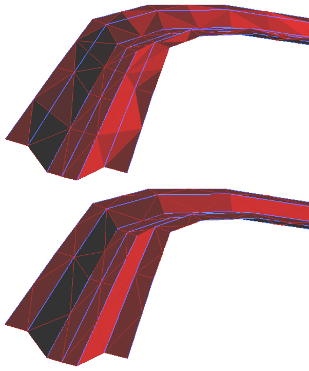
c04f006.tif — **Figure 4-6:** The effect of breaklines on a surface

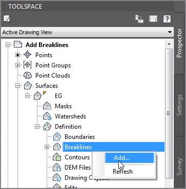
c04f007.tif — **Figure 4-7:** Adding breaklines from within Prospector

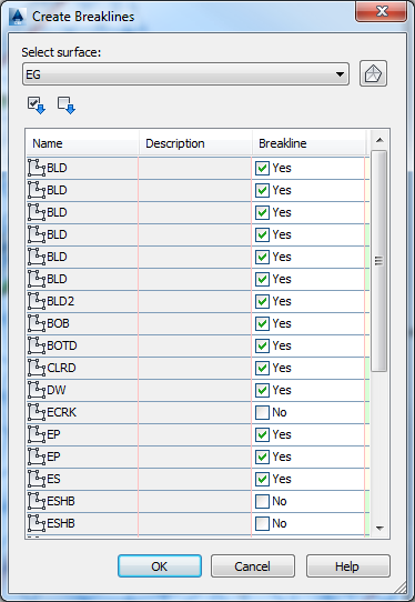
c04f008.tif — **Figure 4-8:** Creating breaklines from survey figures. Note how some figures are checked as breaklines and some are not.

Exercise 4.2: Add Breaklines

In this exercise, you’ll add breaklines to a surface and observe their effect on the accuracy of the surface.

Open the drawing named Add Breaklines.dwg located in the Chapter 04 class data folder.
On the Survey tab of the Toolspace, right-click Survey Databases and select Set Working Folder.
Browse to and select the Chapter 04 class data folder. Click OK. You should see a different survey database named Essentials.
Right-click the Essentials survey database, and select Open For Edit.
Expand the Essentials database. Right-click Figures, and select Create Breaklines.
Scan the list of figures, and note which ones are tagged as breaklines. Click OK.
In the Add Breaklines dialog box, change the Mid-ordinate Distance value to 0.03, and click OK.

Breaklines in the Field

As you study the list of figures in this exercise, are you wondering why some are designated as breaklines and others are not? Breaklines are linear features that mark a change in the slope of the ground. Some of these are quite obvious, such as a set of bottom of bank (BOB) points or top of ditch (TOPD) points. Others serve double duty, such as an edge of pavement (EP). This survey figure marks the line where pavement ends and dirt begins, but typically there is also a change in slope at this line between the slope of the ground and the manmade slope of the road. For this reason, EPs are often tagged as breaklines. Other features obviously have nothing to do with the slope of the ground, such as a right of way (ROW), treeline (TL), and fence line (FENC); therefore, they aren’t checked as breaklines.

You should notice a change in the contours along the red breaklines. These breaklines define the swales, edges, and ridges that were recognized in the field and explicitly located as terrain features. In addition, notice that contours now cover the road area to the north. The surface in this area is made strictly of breaklines.
In the top-right viewport, click one of the surface contours, and then click Surface Properties on the ribbon.
On the Information tab of the Surface Properties dialog box, change Surface Style to Triangles. Click OK. Notice how TIN lines don’t cross the breaklines.
Open Surface Properties again. On the Definition tab, uncheck the box next to Add Breakline, as shown in Figure 4-9. Click OK, and then click Rebuild The Surface.

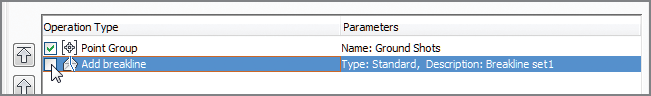
Figure 4-9: Unchecking the Add Breakline operation for the surface

You have removed the effect of the breaklines temporarily. Notice how the TIN lines cross back and forth over the swale and ridge lines, creating a rough edge where there should be a sharp, well-defined edge.
Save and close the drawing.

You can view the results of successfully completing this exercise by opening Add Breaklines - Complete.dwg.

This exercise shows you the importance of breaklines. Connecting a bunch of points together with 3D triangular shapes does not necessarily generate an accurate surface. In certain areas, the shapes themselves have to be manipulated so that they align with terrain features in order to model their form accurately. Figure 4-10 compares the surface with and without breaklines in both 2D and 3D views.

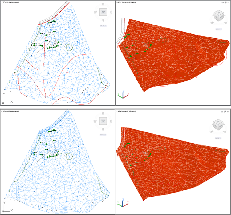
c04f010.tif — **Figure 4-10:** The two top views show the surface in 2D and 3D without the breaklines; the two bottom views show the surface with the breaklines included.

Breakline Settings and Options

The Add Breaklines dialog box has several options and values to choose from. Here is a brief explanation of each:

Type Of the five types listed here, only two are important to discuss at this time: proximity and standard. Standard breaklines have two jobs. First, they control the alignment of TIN lines, as discussed previously. Second, their vertices are a source of additional point information in the drawing. As you might recall, the only point group you added to the surface is Ground Shots, so you’ll need the points to come along with any breaklines you add. For this to work, the vertices of the breaklines must be 3D and must be at the correct elevations.

Proximity breaklines have only one job, which is to control the alignment of TIN lines. Therefore, proximity breaklines only need to be 2D, but they must have points in their proximity so that they can “steal” their elevations. If you had added all the survey points to your surface, then the survey figures could have been added as proximity breaklines.

Weeding Factors Sometimes, the items you use for breaklines can have too many vertices on them, and you’ll want to eliminate some of them so that your surface isn’t overloaded with data. The selective removal of points based on distance and angle is known as weeding.
Supplementing By Distance Sometimes your breaklines will have long stretches without any vertices in them. Because new TIN lines are created only where there are points, and points are created only where there are vertices, some supplemental vertices may be needed to improve the accuracy of the surface. When you check the box next to Distance, Civil 3D creates more points along the breakline that are spaced out according to the value you provide.
Supplementing By Mid-Ordinate Curves are a bit of a challenge because TIN lines are straight and curves are, well, curved. For that reason, any curves in a breakline are approximated with a series of short TIN lines. Just how short and numerous these lines are depends on the mid-ordinate setting. Mid-ordinate is a geometric term that refers to the perpendicular distance between an arc and its chord. When this distance is short, the chord is also short, and multiple instances of it can fit within the length of the arc. This might seem like a strange way to define this behavior, but what’s handy about it is that a single mid-ordinate value works pretty well for a fairly wide range of curve radii. The following image shows the effect of the mid-ordinate setting on a surface. The image on the left uses a value of 0.1, and the image on the right uses a value of 1.0.

Editing Surfaces

With the inclusion of points and breaklines in the surface, you have essentially provided all the data that will be needed to create the surface model. However, you should continue manipulating this data until you achieve the most accurate representation possible of the existing ground surface. You can edit surfaces in many ways. In the following sections, you’ll learn about three surface-editing methods: adding boundaries, deleting lines, and editing points.

Adding Boundaries

As discussed earlier, boundaries are a way of defining where the surface is and where it isn’t. In the example project, you don’t want the surface to exist outside the area that has been surveyed. Why would the surface extend beyond the survey data? If the edge of an area represented by the points happens to bend inward, the lines will extend across the “bay” (see Figure 4-11) and will create misrepresented surface data in that area. One way to avoid or correct this situation is to provide an outer boundary that prevents the surface from existing in these areas.

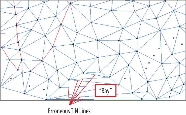
c04f011.eps — **Figure 4-11:** Erroneous TIN lines created across a bay in the surface data

Another common example of surfaces being where they shouldn’t be is within the shape of a building. It’s considered poor drafting practice to show contours passing through a building. After all, the ground surface isn’t accessible in that location. Another type of boundary, called a hide boundary, can be used to remove surface data from within a surface, thus creating a void or “hole” in the surface.

Types of Boundaries

The four types of boundaries you can create with Civil 3D are as follows:

Outer An outer boundary establishes a perimeter for the surface. No surface data can exist outside an outer boundary. This type of boundary is commonly used in most surfaces.

Hide A hide boundary creates a void or “hole” in the surface. Hide boundaries are commonly used to remove surface data within buildings.
Show A show boundary creates an island of data within a hide boundary. An example of a show boundary is a courtyard within the footprint of a building.
Data Clip The first three types of boundaries hide the surface data after it has been created. A data-clip boundary is a special type of boundary that prevents data outside it from ever becoming part of the surface. Data-clip boundaries are used in cases where a small surface is made from source data that covers a large area.

Exercise 4.3: Add Boundaries

In this exercise, you’ll add boundaries around the buildings that will remove surface data from within their footprints.

Open the drawing named Surface Boundaries.dwg located in the Chapter 04 class data folder.
Click one of the surface contours in the top-right viewport. Then, on the Tin Surface: EG tab of the ribbon, click Add Data ⇒ Boundaries.
Enter Bld1 as the boundary name, and select Hide as the type. Make sure the box next to Non-Destructive Breakline is checked, and click OK.

The Non-Destructive Breakline option creates a clean edge along the boundary by trimming some TIN lines and adding others.
Select one of the buildings in the top-right viewport, and press Enter.
This is the effect we’re looking for with separating info for instruction. You should immediately see a hole appear in the surface shown in the lower-right viewport. If you’ve selected a building with contours running through it, you’ll see the contours disappear in the upper-right viewport. It appears that they have been trimmed, but actually, the surface data has been removed from within the shape of the building.
Repeat steps 2 to 4 for the other buildings, even if contours don’t pass through them. Use a name other than Bld1, or the software won’t accept your boundaries.
In the lower-right viewport, zoom in to the area of the buildings, and notice that there are now voids where the buildings are located, as shown in Figure 4-12.

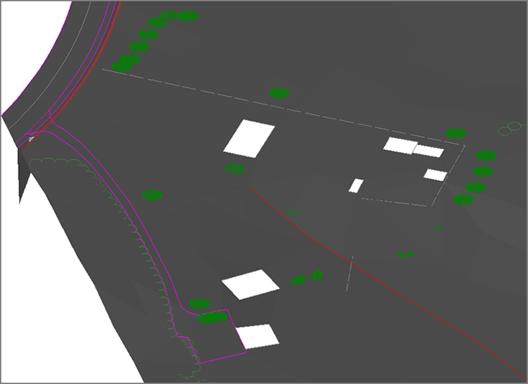
Remember that contours aren’t the only things surfaces are used for. No matter how you look at this surface, you don’t want data to appear where the buildings are.

Figure 4-12: The effect of hide boundaries added at building locations
Save and close the drawing.

You can view the results of successfully completing this exercise by opening Surface Boundaries - Complete.dwg.

Deleting Lines

Another, less eloquent way of removing unwanted TIN lines is to delete them from the surface rather than use a boundary to do it for you. This method is best when you need to remove only a few TIN lines in isolated areas. There are two important things to remember when deleting TIN lines. First, in order for the lines to be deleted, they must be visible, which means you must apply a style that displays them. Second, you can’t use the AutoCAD ERASE command to remove them; instead, you must use the Delete Line command created especially for surfaces.

Exercise 4.4: Delete Lines

In this exercise, you’ll delete unwanted TIN lines from the surface.

Open the drawing named Delete TIN Lines.dwg located in your Chapter 04 class data folder.
Click one of the contours in the top-right viewport, and then select Surface Properties on the ribbon.
On the Information tab, change Surface Style to Triangles and click OK. Press Esc to clear the selection of the surface.
In the left viewport, zoom in to the southern edge of the surface, and note the TIN lines that extend across the bend in the stream (shown previously in Figure 4-11).
Select one of the TIN lines, and then click Edit Surface ⇒ Delete Line on the ribbon. Select the erroneous lines as indicated previously in Figure 4-11. Press Enter after you’ve made your selection.
Pan around the edge of the surface, and delete any other TIN lines that look like they don’t belong. The resulting surface should look similar to Figure 4-13.

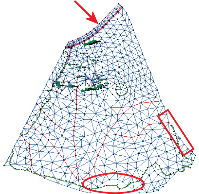
Figure 4-13: The extents of the surface after erroneous TIN lines have been removed. The areas of removal are highlighted.
Save and close the drawing.

You can view the results of successfully completing this exercise by opening Delete TIN Lines - Complete.dwg.

Editing Points

As you have learned, the fundamental building blocks of surfaces are points and lines. The points are derived from some other source of data, such as standard breaklines, contours, survey points, and so on. If there is an error in one of those source objects, there will be an error in the surface as well. When this occurs, you can either edit the source data and rebuild the surface, or edit the surface itself.

Exercise 4.5: Edit Points

You have already learned about editing survey source data (survey points and survey figures). In this exercise, you’ll edit the surface.

Open the drawing named Editing Points.dwg located in your Chapter 04 class data folder.
The two right viewports are zoomed in to the location where the driveway meets the road on the north side of the property. In this area, one of the surface points is incorrect. In the plan view on the top right, the effects of the incorrect point can be seen in the densely packed contours. In the 3D view on the bottom right, the erroneous point appears as a downward spike in the surface.
Click one of the contours to select the surface, and then click Surface Properties on the ribbon.
In the Surface Properties dialog box, click the Information tab and change Surface Style to Triangles And Points. Click OK.
The display of the surface changes to lines and points, with the points appearing as plus-sign markers.
Click any TIN line to select the surface, and then click Edit Surface ⇒ Modify Point on the ribbon.
When prompted to select a point, click the point in the 3D view that is located well below the other points (see Figure 4-14). Press Enter.
At the command line, type 190.76 (58.144), and press Enter.
Notice how the surface is modified but the survey figure is left behind. Depending on the situation, it may be prudent to go back to the source data for the survey figure and correct that as well.

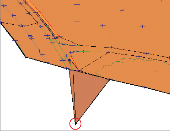
Figure 4-14: 3D view of incorrect surface point
Press Enter to exit the Modify Point command. Change the style of the surface back to C-Existing Contours (1') (C-Existing Contours (0.5m)).
Notice that the closely spaced contours in the top-right viewport are no longer there.
Save and close the drawing.
You can view the results of successfully completing this exercise by opening Editing Points - Complete.dwg.

Displaying and Analyzing Surfaces

Because you’re working with surface objects in Civil 3D, you can do much more than simply show contours. Civil 3D surfaces can help you tell many different stories about the shape of the land and how water will flow across it. They are able to do this through multiple types of analyses as well as the ability for styles to display analysis results in nearly any way you wish. With these tools at your disposal, you can study the terrain thoroughly and make smart choices about the direction of your design early in the process.

Analyzing Elevation

Elevation analysis allows you to delineate any number of elevation ranges and then graphically distinguish the different ranges by color. This is a useful tool in many instances, especially when you’re working with someone who doesn’t know how to read contours.

Exercise 4.6: Analyze Elevation

In this exercise, you’ll perform an elevation analysis on a surface in your drawing.

Open the drawing named Elevation Analysis.dwg located in the Chapter 04 class data folder.
Click one of the contours to select the surface, and then click Surface Properties on the ribbon.
Change Surface Style to Elevation Banding (2D).
Click the Analysis tab. Verify that the analysis type is Elevations and the number of ranges is 8.
Click the downward-pointing arrow to populate the Range Details section of the dialog box with new data.
Click OK to return to the drawing. Press Esc to clear the selection of the surface.
The surface undergoes an obvious change, and it’s now displayed as a series of colored bands with red signifying the lowest elevations and purple signifying the highest.
Change the style of the surface to Elevation Banding (3D).

You may need to zoom out a bit in the lower-right viewport to see the 3D color representation of the surface.

Now the 3D view displays the colored bands as a 3D representation with exaggerated elevations. This tells a clear story about the existing shape of the land for this site (see Figure 4-15).

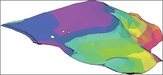
Figure 4-15: A 3D view of a surface using the Elevation Banding (3D) style
Save and close the drawing.

You can view the results of successfully completing this exercise by opening Elevation Analysis - Complete.dwg.

Analyzing Slope

Another important aspect of the terrain is the slope. Areas with very steep slopes are difficult to navigate either by construction vehicles or the eventual occupants of the property. Flat slopes are much more accessible, but if they are too flat, then drainage problems often occur. One of your tasks as a designer is to ensure that your project has the right slopes in the right areas. By studying the slopes of the existing topography, you can locate features where slopes are good or determine that terrain modifications will be necessary to create good slopes.

Civil 3D can display slopes in two ways. The first is to show the slopes as colored ranges like the ones you saw in the previous section. The second is to use slope arrows that can be color coded to indicate in what range they’re located, with the added benefit of always pointing downhill to show you the direction of water flow.

Exercise 4.7: Analyze Slope

In this exercise, you’ll perform a slope analysis on a surface in your drawing.

Open the drawing named Slope Analysis.dwg located in the Chapter 04 class data folder.
Click one of the contours to select the surface, and then click Surface Properties on the ribbon.
On the Information tab of the Surface Properties dialog box, change Surface Style to Slope Banding (3D).
Click the Analysis tab. Change Analysis Type to Slopes, and click the downward-pointing arrow.
Click OK. Press Esc to clear the selection of the surface and zoom in to the 3D view of the surface in the bottom-right viewport.
In the 3D image on the bottom right, the darkest reds signify the steepest slopes. This enables you to see that the area north of the farm is fairly flat pasture land while the area to the south of the farm slopes dramatically toward the stream farther to the south (see Figure 4-16).
Access Surface Properties again, and change the style to Slope Arrows.

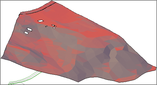
Figure 4-16: Slope analysis of surface shown in 3D
On the Analysis tab, choose Slope Arrows as the analysis type, and click the arrow again.
Click OK to return to the drawing. Press Esc to clear the selection of the surface.
In this view, the darker blues and blacks are the steepest slopes, and the arrows themselves always point downhill. As you study the arrows, you should notice a drainage divide that runs west to east through the farm buildings; it’s delineated in red in Figure 4-17. Rain falling to the north of this area drains to the road, and rain falling south of it drains to the stream.

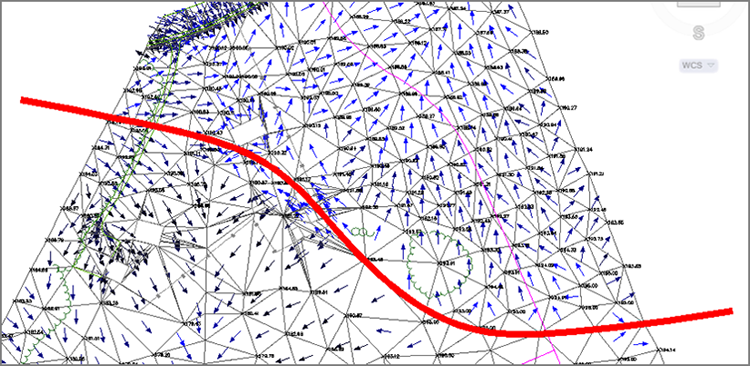
Figure 4-17: Slope arrows can be used to identify a drainage divide (delineated in red) in the project.
Save and close the drawing.
You can view the results of successfully completing this exercise by opening Slope Analysis - Complete.dwg.

Performing Other Types of Analysis

In addition to analyzing elevations, slopes, and slope arrows, you can perform the following types of analyses:

Contours Contours can be used to analyze a surface. They can be color coded, and you can create a legend table that shows the area and/or volume the contours represent.
Directions With this type of analysis, you can see a visual representation of your surface slopes. For example, you can use the analysis to see which parts of your surface slope to the south and which slope to the north.
User-Defined Contours Contours are usually placed at even intervals, such as the 1' (0.5 meter) contours with which you have been working so far. What if you want to show a contour that represents elevation 92.75? That’s done as a user-defined contour. A user-defined contour is an individual instance of a contour, usually at an irregular interval.
Watersheds A watershed analysis outlines areas within the surface where rainfall runoff flows to a certain point or in a certain direction. This type of analysis is yet another way of studying the drainage characteristics of the terrain.

Exploring Even More Analysis Tools

There are even more ways of analyzing your surface that aren’t found in Surface Properties. For example, the following tools are especially useful on many projects:

Water Drop Tool With the Water Drop tool, you can click any point on your surface and Civil 3D will trace the path from that point downhill until it reaches a low point or encounters the edge of the surface. This is a very detailed way to study how water will flow across the ground.
Catchment Area Tool With this tool, you can click a point on the surface and Civil 3D will draw a closed shape that represents the area that flows to that point. This is very useful when you’re analyzing the effects of rainfall on your project.
Quick Profile With the Quick Profile tool, you can display a slice of your surface to get an edge-on view of it. This can help you understand the slope of the land and the location of high and low points.

You’ll learn more about these tools and get hands-on experience with them in Chapter 18, “Analyzing, Displaying, and Annotating Surfaces.”

Annotating Surfaces

As you have read, surfaces are used to tell a story about the shape of a piece of land. I have presented nearly a dozen different ways to tell that story, but I have yet to discuss the most obvious and most common way: telling the story with text. In the following exercise, you’ll use three types of labels to annotate a surface: spot elevation labels, slope labels, and contour labels.

Exercise 4.8: Annotate a Surface

In this exercise, you’ll annotate a surface using spot elevation labels, slope labels, and contour labels.

Open the drawing named Labeling Surfaces.dwg located in the Chapter 04 class data folder.
The top-right viewport is zoomed in to the north end of the project near the location where the magenta centerline meets the centerline of the existing road. Your task is to label the elevation of the existing road where these two centerlines meet.
Click one of the contours to select the surface, and then click Add Labels ⇒ Add Surface Labels on the ribbon.
In the Add Labels dialog box, select Spot Elevation as the label type.
Verify that the spot elevation label style is set to Elevation Only – Existing and the marker style is set to Spot Elevation.
Click Add. Snap to the northern endpoint of the magenta centerline. A label is placed at the location you selected (see Figure 4-18).
Pan to the south where the road centerline bends at a 90-degree angle.
Note the steep slope to the south of the road in this area. You want to measure and label the slope in this area to determine whether homes can be built here and/or if guardrails will be required for the road.
If the Add Labels dialog box is already open, skip to the next step. If not, click one of the contours to select the surface, and then click Add Labels ⇒ Add Surface Labels on the ribbon.

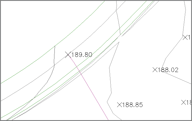
Figure 4-18: Spot elevation label showing 189.80' (57.85m) added where the new road meets the existing road
For Label Type, select Slope.
Verify that Slope Label Style is set to Percent-Existing, and click Add.
When prompted at the command line, press Enter to accept the default of <One-point>.
Click a point to the south of the road to label the slope. Press the Esc key to end the command.

This creates a label that points downhill at the one point you select. With two-point labels, you control the direction.
Click the label, and then click the square grip at the midpoint of the arrow. Move your cursor across the drawing, and note how the label changes.

This dynamic label behavior is consistent throughout Civil 3D.
If the Add Labels dialog box is already open, skip to the next step. If not, click one of the contours to select the surface, and then click Add Labels ⇒ Add Surface Labels on the ribbon.
For Label Type, select Contour – Multiple. Verify that the names of all three label styles begin with Existing, and click Add.
Click two points in the drawing that stretch across several contours.
Contour labels appear where contours fall between the two points you’ve selected (see Figure 4-19). You’ve actually drawn an invisible line that intersects with the contours.
Press Esc to clear the previous command, and then click one of the newly created labels.
Notice the line that appears. Click one of the grips, and move it to a new location to change the location of the line. The contour labels go where the line goes, even if you stretch it out and cause it to cross through more contours, in which case it will create more labels.

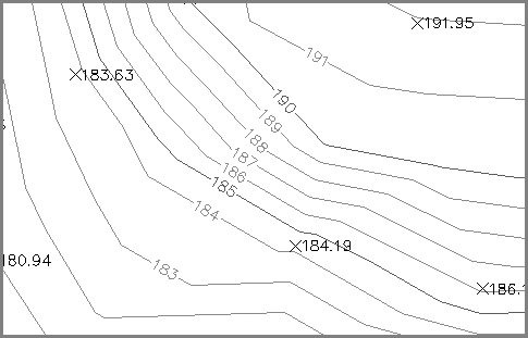
Figure 4-19: Contour labels
Continue placing contour labels until you’ve evenly distributed labels throughout the drawing.
Save and close the drawing.
You can view the results of successfully completing this exercise by opening Labelling Surfaces - Complete.dwg.

Now You Know

Now that you have completed this chapter, you understand the role of surfaces in land-development projects. You can create surfaces from survey data and perfect them by adding breaklines and boundaries. You can modify surfaces by deleting lines and editing points. You can get answers and tell stories about surfaces using analysis types such as elevation banding, slope banding, and slope arrows. Finally, you’re able to provide additional information about a surface using several different types of labels.

Now that you’ve learned this major step in establishing the existing conditions of your project, you’re ready to begin learning about the tools used to transform your project through design.