Chapter 8
Displaying and Annotating Profiles

Now that you have captured the nature of the existing ground along the road centerlines using surface profiles, and you have reshaped it using layout profiles, it’s time to specify how you intend your design to be built. A wavy line in the drawing simply isn’t enough information for a contractor to start building your design. You need to provide specific geometric information about the profile so that it can be re-created in the field. This is done with various types of annotations available in the AutoCAD^® Civil 3D^® software.

It’s also important that the framework in which the profiles are displayed is properly configured. As you learned in the previous chapter, the grid lines and grid annotations behind your profiles form a profile view. In this chapter, you’ll look at applying different profile view styles to control what information about your profiles is displayed and in what manner.

Finally, it’s often necessary to show other things in a profile view that might impact the construction of whatever the profile represents. Pipe crossings, underground structures, rock layers, and many other features may need to be displayed so that you can avoid them or integrate your design with them. One way of showing these items in your profile view is through a Civil 3D function called object projection.

In this chapter, you’ll learn to

Change the display of profiles with profile styles
Configure profile views using profile view styles
Share information through profile view bands
Add detail using profile labels
Work efficiently using profile label sets
Add detail using profile view labels
Project objects to profile views

Applying Profile Styles

As with any object style, you can use profile styles to show profiles in different ways for different purposes. Specifically, you can use profile styles to affect the appearance of profiles in three basic ways. The first is to control which components of the profile are visible. You might be surprised to know that there are potentially eight different components of a profile. The second is to control the graphical properties of those components, such as layer, color, linetype, and so on. Finally, a profile style enables you to control the display of markers at key geometric points along the profile. Once again, you might be surprised at the number of types of points that can be marked along a profile: there are 11 of them.

Exercise 8.1: Apply Profile Styles

In this exercise, you’ll assign different profile styles to a profile and observe the different ways profiles can be represented.

Open the drawing named Profile Styles.dwg located in the Chapter 08 class data folder.

Be sure your background color is set to white before proceeding with these steps.
In the Jordan Court profile view, click the red existing-ground profile, and then click Profile Properties on the ribbon.

Because the majority of the work in this chapter is done in profile view, the drawings aren’t set up with multiple viewports.
On the Information tab of the Profile Properties dialog box, change the style to _No Display. Then click OK.
The profile disappears from view.
Press Esc to clear the selection of the existing ground profile. Then click the black design profile for Jordan Court. Right-click, and select Properties.
In the Properties window, change the Style property to Layout, and press Esc to clear the grips.

You can also use the specific Profile Properties command to access the style assignment. To show it a different way, however, in step 5 you use the generic Properties command instead.

The profile now shows curves and lines as different colors and includes markers that clearly indicate where there are key geometry points (see Figure 8-1). This might be helpful while you’re in the process of laying out the profile, but it may not work well when you’re using the profile to create a final drawing.

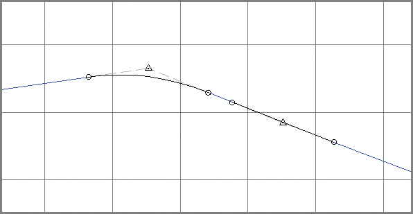
Figure 8-1: The Layout profile style displays lines and curves with different colors as well as markers at key geometric locations.
Select the Jordan Court profile again. In the Properties window, change the style to Basic.

This is a very simple style that shows just the basic geometry with no markers or color differences.

Using a Style to Hide an Object

In step 3 in Exercise 8.1, you use the style _No Display to hide the profile—something you might normally do by turning off or freezing a layer. This method of making things disappear via style is used quite a bit in Civil 3D. In fact, if you look in the stock template that ships with Civil 3D, you’ll see a _No Display style for nearly every object type.

Using this approach has a couple of advantages over turning layers on and off. First, many Civil 3D objects have multiple components that can be displayed on different layers. Changing one style is more efficient than changing several layers, so it becomes easier and quicker to control the visibility of components by style. Second, you may not know which layer or layers need to be turned off to make the object disappear from view. By simply applying the _No Display style, you make the items disappear without considering layers at all.
Change the style to Design Profile With Markers.

This style displays the lines and curves on the standard road profile layer, includes markers that are typically used for annotation, and shows the line extensions as dashed lines. This style is an example of how you might represent a profile in a final drawing.
In Prospector, expand Alignments ⇒ Centerline Alignments ⇒ Jordan Court ⇒ Profiles. Right-click Jordan Court EGCL and select Properties, as shown in Figure 8-2.

Remember that this profile was set to _No Display so we can’t pick it in the drawing. One way to get to it is through the Prospector tab.
Change the style to Existing Ground Profile, and click OK so the drawing it looks like it did when you started this exercise.
Save and close the drawing.

You can view the results of successfully completing this exercise by opening Profile Styles - Complete.dwg.

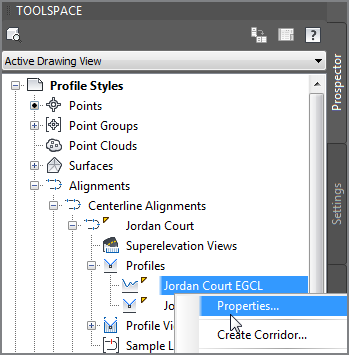
c08f002.tif — **Figure 8-2:** Using Prospector to access the Properties command for the Jordan Court EGCL profile

Applying Profile View Styles

Styles are especially important when you’re working with profile views because of their potential to dramatically affect the appearance of the data that is being presented. Among other things, profile view styles can affect vertical exaggeration, spacing of the grid lines, and labeling.

Exercise 8.2: Apply Profile View Styles

In this exercise, you’ll assign different profile view styles and observe how they can change the way profile information is presented.

Open the drawing named Profile View Style.dwg located in the Chapter 08 class data folder.
Click one of the grid lines of the Jordan Court profile view, right-click, and select Properties.

10V refers to a vertical exaggeration that is 10 times that of the horizontal. Note that in the Properties window, the current profile view style is named Major Grids 10V.
In the Properties window, change the style to Major & Minor Grids 10V. Press Esc to clear the selection.
Note the additional grid lines that appear (see Figure 8-3).
Select the profile view grid, and change the style to Major Grids 5V.
With this change, the vertical exaggeration is reduced to 5. This makes the profile appear much flatter.
Change the style to Major Grids 1V.

This displays the profile in its true form, as it really exists in the field. Think about which profile would be easier to work with: the exaggerated one, where the peaks and valleys are obvious, or this one, which is true to scale but much more difficult to analyze?

Figure 8-3: Additional grid lines displayed as a result of applying the Major & Minor Grids 10V profile view style

It’s OK to Exaggerate Sometimes

Vertical exaggeration is a common practice used to display information in profile view. In most places, the earth is relatively flat, and changes in elevation are subtle. To make the peaks and valleys stand out a bit more, the elevations are exaggerated while the horizontal distances are kept the same. The result is a profile that appears to have higher high points, lower low points, and steeper slopes in between. This makes the terrain easier to visualize and analyze. When this technique is used, you’ll likely see a pair of scales assigned to the drawing: one that represents the horizontal scale and one that represents the vertical scale. For example, a drawing that has a horizontal scale of 1" = 50' and a vertical scale of 1" = 5' is employing a vertical exaggeration factor of 10. For a metric example, a horizontal drawing scale of 1:500 and a vertical drawing scale of 1:50 also achieves a vertical exaggeration of 10.

The following three profile views have a vertical exaggeration of 10, 5, and 1, from left to right. The same existing ground profile is shown as a red line in all three.
Change the style of the profile view to DOT.

DOT stands for Department of Transportation, which in the United States is a common way of referring to government regulatory departments and other agencies that manage roads and other transportation infrastructure.

This is an example of how the graphical standards of a client or review agency can be built into your Civil 3D standard styles, making it easy to meet the requirements of others.
Save and close the drawing.
You can view the results of successfully completing this exercise by opening Profile View Style - Complete.dwg.

Applying Profile View Bands

Profile view bands can be added to a profile view along the top or bottom axis. You can use these bands to provide additional textual or graphical information about a profile. They can be configured to provide this information at even increments or at specific locations along the profile.

Exercise 8.3: Apply Profile View Bands

In this exercise, you’ll configure bands for the Jordan Court profile view so that information about stations, elevations, and horizontal geometry can be displayed.

Open the drawing named Profile View Bands.dwg located in the Chapter 08 class data folder.
Click one of the grid lines of the Jordan Court profile view, and then click Profile View Properties on the contextual ribbon tab.
On the Information tab of the Profile View Properties dialog box, change Object Style to Major & Minor Grids 10V.

Earlier, you used the AutoCAD^® Properties window to change the profile view style. This is another way to do it.
Click the Bands tab. Verify that Profile Data is selected as Band Type.
Under Select Band Style, choose Elevations And Stations. Then click Add.
In the Geometry Points To Label In Band dialog box, on the Profile Points tab, select Jordan Court EGCL as Profile 1, as shown in Figure 8-4. Click OK.

You may have noticed the long list of geometry points in this dialog box. The band style you have selected doesn’t include references to any of these points; therefore, no geometry point information will appear on the band.

A new entry is added to the list of bands.

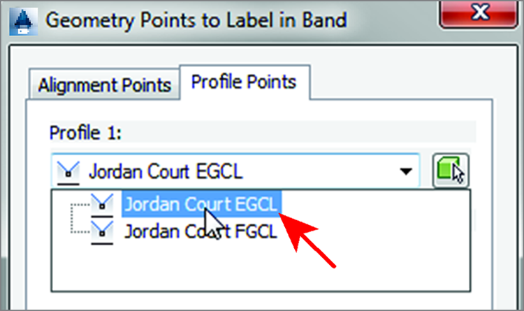
Figure 8-4: Assigning Jordan Court EGCL as Profile 1
In the Profile View Properties dialog box, scroll to the right until you see the Profile 2 column. Click the cell in this column, and select Jordan Court FGCL.
Click OK to dismiss the Profile View Properties dialog box and return to the drawing. Zoom in to the bottom of the profile view.

This band is designed for two profiles, so there are two sets of elevations. The elevations on the left side of each line refer to the Jordan Court EGCL profile, and the ones on the right side refer to the Jordan Court FGCL profilend.

Across the bottom of the profile view, there is now a band that labels the stations and elevations at even increments (see Figure 8-5).

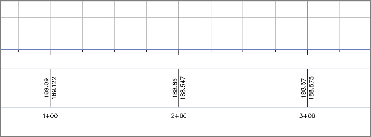
Figure 8-5: The newly added band showing stations, existing elevations (left), and proposed elevations (right)
Click the profile view, and select Profile View Properties from the ribbon again.
On the Bands tab, select Horizontal Geometry as Band Type.
Under Select Band Style, choose Geometry, and click Add.

Band Sets

Right after step 7 you could have clicked Save As Band Set and stored the two bands as a new band set. This band set could then be imported into another profile view at a later time. This feature is handy when you repeatedly use the same list of bands, enabling you to avoid rebuilding the list each time.
Click OK to dismiss the dialog box and return to the drawing.
The new band is a graphical representation of the alignment geometry. Upward bumps in the band represent curves to the right, and downward bumps represent curves to the left. The beginning and ending of each bump corresponds with the beginning and ending of the associated curve. There are also labels that provide more specifics about the horizontal geometry.
Click the Jordan Court profile view; then click Profile View Properties on the ribbon.
On the Bands tab, click the Horizontal Geometry band entry, and then click the red X icon to remove it.
Click OK to return to the drawing.

The Horizontal Geometry band is removed from the bottom of the Jordan Court profile view.
Save and close the drawing.

You can view the results of successfully completing this exercise by opening Profile View Bands - Complete.dwg.

Applying Profile Labels

Profile labels are similar to alignment labels. They’re applied to the entire profile or to a range within the profile, and they show up wherever they encounter the things they’re supposed to label. For example, if a vertical curve label is applied to a profile that has three vertical curves, then three vertical curve labels will appear. This approach offers two advantages. The first is that you can label multiple instances of a geometric feature with one command. This becomes significant when you’re working on a long stretch of road with dozens of vertical curves. The other advantage is that labels appear as new geometric features are added. Continuing to use vertical curves as an example, if you apply a vertical curve label to a profile, curve labels will appear or disappear automatically whenever you create or delete vertical curves.

Exercise 8.4: Apply Profile Labels

In this exercise, you’ll configure the labels for the Jordan Court design profile so that tangent grades and curve data are labeled.

Open the drawing named Profile Labels.dwg located in the Chapter 08 class data folder.
Click the Jordan Court FGCL profile, and then click Edit Profile Labels on the ribbon.
In the Profile Labels – Jordan Court FGCL dialog box, select Crest Curves as Type.

Refer to the section, “Profile Terminology,” in Chapter 7 to review information about crest curves and sag curves.
Select Crest Only for Profile Crest Curve Label Style, and then click Add.
Click OK to return to the drawing. All the crest curves in the profile are labeled.
Click the Jordan Court FGCL profile, and then click Edit Profile Labels on the ribbon again. Add the following profile labels:

Type Style

Sag Curves Sag Only

Lines Percent Grade

Grade Breaks Station over Elevation

The list of labels should appear as shown in Figure 8-6.

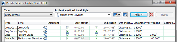
Figure 8-6: The list of labels to be applied to the Jordan Court FGCL profile
Click OK to close the Profile Labels – Jordan Court FGCL dialog box and return to the drawing. Press Esc to clear the selection in the drawing.

The profile is now annotated with several types of labels. Some of the label positions need to be adjusted to improve readability, which you’ll do next.
Zoom in to the third curve label from the left.

Notice how the curve-length dimension line is crossing through the profile.
Click the label to show its grips. Then click the diamond-shaped grip at the base of the dimension text, and move it up until the label is more readable.
Repeat step 9 for any other curve labels that need to be moved to improve readability.
Save and close the drawing.

You can view the results of successfully completing this exercise by opening Profile Labels - Complete.dwg.

Creating and Applying Profile Label Sets

In the previous exercise, you used several types of profile labels to annotate the design profile for Jordan Court. Each one had to be selected and added to the list of labels, making this a multistep process. A profile label set enables you to store a list of labels for use on another profile. The settings for each label—such as weeding, major station, minor station, and so on—can also be stored in the label set. This is quite helpful if you use the same profile labels for multiple profiles. A label set can even be stored in your company template so it’s always there for you to use.

Exercise 8.5: Apply Profile Label Sets

In this exercise, you’ll use a label set to capture the label configuration for Jordan Court and apply it easily to Logan Court.

Open the drawing named Profile Label Set.dwg located in the Chapter 08 class data folder.
Click the Jordan Court FGCL profile, and click Edit Profile Labels on the ribbon.
In the Profile Labels – Jordan Court FGCL dialog box, click Save Label Set to open the Profile Label Set – New Profile Label Set dialog box.
Click the Information tab, and enter Curves-Grades-Breaks for Name. Click OK twice to return to the drawing.
Press Esc to clear the selection of the Jordan Court FGCL profile. Zoom to the Logan Court profile view. Click the Logan Court FGCL profile, and select Edit Profile Labels on the ribbon.
In the Profile Labels – Logan Court FGCL dialog box, click Import Label Set.
Select Curve-Grades-Breaks in the Select Label Set dialog box, and then click OK. Click OK to dismiss the Profile Labels dialog box and return to the drawing.

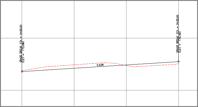
No curve labels appear on the profile because there are no curves. However, if a curve were added, a curve label would appear.

Figure 8-7: Logan Court FGCL profile after the newly created profile label set has been applied

Two grade-break labels and a grade label have been added to the Logan Court FGCL profile (see Figure 8-7).
Save and close the drawing.

You can view the results of successfully completing this exercise by opening Profile Label Set - Complete.dwg.

Creating Profile View Labels

You have just seen how useful profile labels can be because they are applied to the entire profile and continuously watch for new geometric properties to label. However, this dynamic nature may not be ideal in certain situations, or you may need to provide annotation in your profile view that isn’t related to any profiles in that view. Profile view labels are the solution in this case.

Profile view labels are directly linked to the profile view: the grid, grid labeling, and bands that serve as the backdrop for one or more profiles. Because of this, you can use labels that are independent of any profiles. For example, you might use a station and offset label to call out the location of a pipe crossing through the profile view. Because the pipe crossing isn’t directly affected by any profile in the drawing, it wouldn’t make sense to associate this label with a profile. Instead, you would use a profile view label that is specifically intended for the pipe crossing.

Three types of profile view labels are available in Civil 3D: station elevation, depth, and projection. You’ll work with the first two in the next exercise, and the third will be covered later in this chapter.

Exercise 8.6: Apply Profile View Labels

In this exercise, you’ll use profile view labels to label the location where Jordan Court ties in to Emerson Road, including the identification of the ditch area.

Open the drawing named Profile View Labels.dwg located in the Chapter 08 class data folder.
This drawing is zoomed in to the left end of the Jordan Court FGCL profile. At this location, there is a PVI where the new road ties to the edge of the existing road. There is also a V shape in the existing ground profile that shows the existence of a roadside drainage ditch (see Figure 8-8).

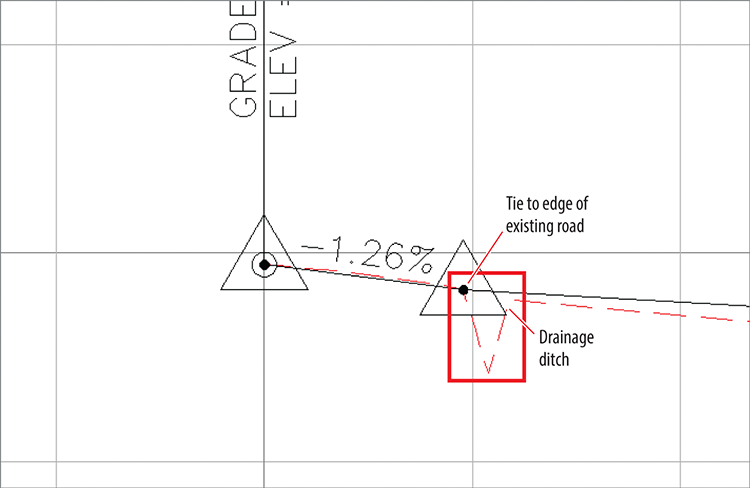
Figure 8-8: The beginning of the Jordan Court FGCL profile, where there is a tie to the edge of the existing Emerson Road as well as a V-shaped drainage ditch
Click one of the grid lines for the Jordan Court profile view. On the ribbon, click Add View Labels ⇒ Station Elevation.
While holding down the Shift key, right-click and select Endpoint from the context menu.
Click the center of the black-filled circle at the second PVI marker.
Repeat the previous two steps to specify the same point for the elevation.

You must provide the location in two separate steps: First you specify the station (step 4), and then you specify the elevation (step 5).

A new label appears, but it’s overlapping the grade label to the left.
Press Esc twice to clear the selection of the profile view and end the command. Then click the newly created label, and drag the square grip up and to the right.
With the label still selected, click Edit Label Text on the ribbon.

This opens the Text Component Editor.
In the text view window on the right, click just to the left of STA to place your cursor at that location. Press Enter to move that line of text down and provide a blank line to type on.
Click the blank line at the top, type TIE TO EDGE, and press Enter.
Type OF EXIST ROAD.
The Text Component Editor dialog box should now look like Figure 8-9.
Click OK to return to the drawing.

Nearly all Civil 3D labels can be edited in this way.

The label now clearly calls out the station and elevation where the new road should tie to the existing road.

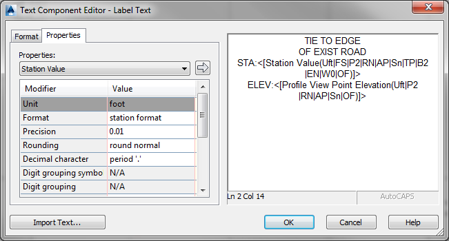
Figure 8-9: Additional text added to a label in the Text Component Editor dialog box
Press Esc to clear the current label selection. Click one of the grid lines of the profile view, and then click Add View Labels ⇒ Depth.
Pick a point at the invert of the V-shaped ditch, and then pick a point just above it approximating the top of the ditch.

Invert is a term referring to the lowest elevation of the ditch. It’s also used to refer to the lowest elevation of a pipe or a structure, such as a manhole or inlet.
Press Esc twice to end the command and clear the selection of the profile view.
Click the newly created depth label, and then click one of the grips at the tip of either arrow. Move the grip to a new location, and note the change to the depth value displayed in the label.
Both the station-elevation label and the depth label can be seen in Figure 8-10.

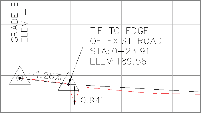
Figure 8-10: The station-elevation label and depth label added to the Jordan Court profile view
Save and close the drawing.
You can view the results of successfully completing this exercise by opening Profile View Labels - Complete.dwg.

Remember Exaggeration?

The roughly 1-foot (0.3-meter) depth shown by the label might seem small to you, based on the dramatic plunge of the V in the profile. Remember that this profile view is exaggerated in the vertical aspect by a factor of 10. If you were to measure this same depth using the DISTANCE command, you would get about 10 feet (3 meters). Profile view labels automatically factor in the vertical exaggeration of your profile view.

Projecting Objects to Profile Views

At times, it may be necessary or helpful to show more in a profile view than just the existing and finished profiles of your design. Features such as underground pipes, overhead cables, trees, fences, and so on may be obstacles that you need to avoid or features that you need to integrate into your design. Whatever the case, Civil 3D object projection enables you to quickly represent a variety of objects in your profile view and provide the accompanying annotation.

Projecting Linear Objects

When you project an object to a profile view, different things can happen depending on the type of object you have chosen. For linear objects such as 3D polylines, feature lines, and survey figures, the projected version of the object is still linear, but it will appear distorted unless it’s parallel to the alignment. This can be a bit tough to envision, but just imagine a light being shone from behind the object in the direction of the alignment. The projection of this object seen in a profile view would be somewhat like the shadow cast by the object. The parts of it that are parallel to the alignment would appear full length, and the parts that aren’t parallel would appear shortened.

Based on the settings you choose, the elevations that are applied to a projected linear object can vary. For linear objects that are already drawn in 3D, you can choose to use the object elevations as they are. For 2D objects that need to have elevations provided, the elevations can be derived from a surface or profile.

Projecting Blocks and Points

Objects that indicate location—such as AutoCAD points, Civil 3D points, and blocks—are handled a bit differently than linear objects. They are represented with markers or as a projected version of the way they are drawn in plan view. This can lead to a distorted view of such objects because of the common practice of applying a vertical exaggeration to the profile view. The options for assigning elevations to these types of projections are the same as the options for linear objects, with one addition: the ability to provide an elevation manually. This allows you to specify the elevation graphically or numerically; independent of a surface, a profile, or the actual elevation of the object you’ve selected.

Exercise 8.7: Project Objects to Profile View

In this exercise, you’ll use object projection to show a water line on the Jordan Court profile view.

Open the drawing named Object Projection.dwg located in the Chapter 08 class data folder.
Click one of the grid lines of the Jordan Court profile view, and then click Project Objects To Profile View on the ribbon.
Zoom in to the eastern property line, and click the blue 3D polyline representing the water pipe that runs parallel to the eastern property line. Press Enter.
In the Project Objects To Profile View dialog box, verify that Style is set to Basic and Elevation Option is set to Use Object.
Click OK. Pan and zoom to the profile view, and press Esc to clear the selection of the profile view.
The projected version of the water line is shown in the profile view (see Figure 8-11). Note the strange bends in the line around station 12+00 (0+360). These are caused by the alignment turning away from the water pipe at this location, which produces some odd projection angles and distorts the projected appearance of the water pipe.

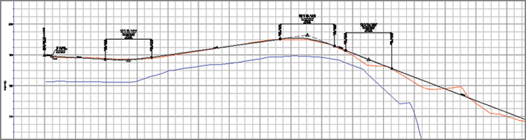
Figure 8-11: A 3D polyline representing a water pipe has been projected into the Jordan Court profile view.
Select the profile view grid for Jordan Court, and click Project Objects To Profile View on the ribbon.
Click three of the points labeled BORE that appear along the Jordan Court alignment. Press Enter.
In the Project Objects To Profile View dialog box, verify that Test Bore is selected as Style and Use Object is selected as Elevation Option for all three points.

The type of style referred to here is a Civil 3D point style. A few steps later, you’ll use a different type of style for a block.
Click OK, and view the projected points in the profile view.
As you can see, the points are inserted with a marker and a label that indicates the station and ground-surface elevation of the test boring (see Figure 8-12).
Press Esc to clear the previous selection. Zoom in near the midpoint of Logan Court, and note the red test-boring symbol shown there.

This is an AutoCAD block, not a Civil 3D point.
Click the profile view for Logan Court, and then click Project Objects To Profile View on the ribbon.

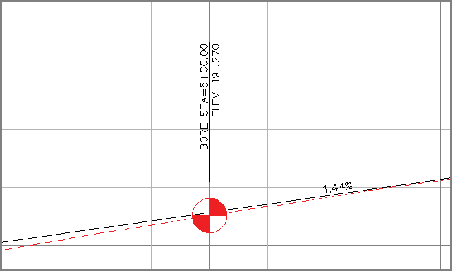
c08f012.tif — **Figure 8-12:** A Civil 3D point projected to the Jordan Court profile view

Click the red test-boring symbol, and press Enter. Verify that Style is set to Basic, and change Elevation Options to Surface ⇒ EG.

Feature lines and Civil 3D points have projection built into their styles, but for AutoCAD entities like this block, an object projection style is used.
Click OK, and examine the new projection added to the profile view.
It looks similar to the projected Civil 3D points, even though the source object in this case is a block with no elevation assigned to it.
Save and close the drawing.

You can view the results of successfully completing this exercise by opening Object Projection - Complete.dwg.

Type	Style
Sag Curves	Sag Only
Lines	Percent Grade
Grade Breaks	Station over Elevation