Chapter 18
Analyzing, Displaying, and Annotating Surfaces

In Chapter 17, “Designing New Terrain,” you experienced a few examples of using the AutoCAD^® Civil 3D^® software to design new terrain in the form of lot grading and pond design. With more time, you would have completed the shaping of all the lots, resulting in a grading design for the entire project. Now that all the major grading design components are complete (roads, lots, and a pond in this example), it’s time to combine them into one complete design. Once you have done this, you can analyze the design to ensure that it meets several additional design and construction requirements. This analysis may result in the need for an adjustment to the design, at which time you’ll begin an iterative process: design, analyze, adjust, design, analyze, adjust, and so on. You’ll repeat this cycle until the design is the best that time and resources permit. When the design is optimized, you can then provide annotation that provides the necessary information for the contractor to build your design for the land’s new shape.

In this chapter, you’ll learn to

Combine design surfaces
Analyze design surfaces
Calculate earthwork volumes
Label design surfaces

Combining Design Surfaces

In Chapter 17, you created a pond design that resulted in a surface representing the shape of the pond. You also performed some lot grading; and if you had continued working on the lot grading for a few hours, you eventually would have finished all the lots, creating a surface that covered nearly the entire project. In Chapter 9, “Designing in 3D Using Corridors,” you created a corridor surface to represent the model of the roads. This approach of designing the shape of the terrain in parts is common and recommended. For even the most talented designer, it’s difficult to design all aspects of a project at once. It’s easier, and often more efficient, to divide the design into “mini-designs” such as the road, lots, and pond that you experienced for yourself.

Once the parts are in place, it’s then time to combine them into one master surface. To accomplish this, you use a simple but very powerful capability of surfaces in Civil 3D: pasting. Just as you’re able to paste a paragraph of text into a document, you can paste one surface into another. The similarities between surfaces and documents end there, however. For example, when you paste one surface into another, the pasted version is a live copy of the original, meaning if the original is modified, the pasted version is also modified. To find the command to paste surfaces, right-click Edits in a surface in Prospector or choose the Surfaces ribbon tab (see Figure 18-1).

c18f001.eps — **Figure 18-1:** The Paste Surface command, located in a Prospector context menu (left) and the Surface ribbon tab (right)

When you’re working with multiple pasted surfaces, you can use the order in which they are pasted to achieve a desired result. The way this works is that when two overlapping surfaces are pasted, the second one overwrites the first in the area where they overlap. You can control the order in which surfaces are pasted on the Definition tab of the Surface Properties dialog box (see Figure 18-2). Here you can rearrange the order of operations not just for pasting surfaces, but for other operations as well.

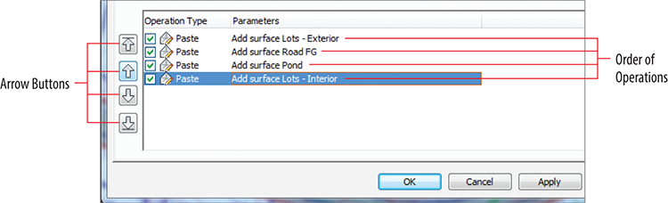
c18f002.eps — **Figure 18-2:** You can change the order of operations using the arrow buttons. This can affect the result of pasting multiple surfaces together.

Exercise 18.1: Combine Surfaces

In this exercise, you’ll create an FG Final surface by combining surfaces representing lot grading, road elevations, pond grading, and a small area of daylighting.

Open the drawing named Combining Surfaces.dwg located in the Chapter 18 class data folder.

Make sure your background color is set to white before completing the exercises in this chapter.

In this drawing, the lot grading design is complete, as shown by the blue, red, and green feature lines. There is also a small area between lots 73 and 76 where a grading group was used to calculate daylighting.
In Prospector, expand Surfaces, and note the surfaces that are listed. Right-click Surfaces, and select Create Surface.

All the surfaces except EG have a style of _No Display assigned to them. That is why no design contours are shown in the drawing.
On the Create Surface dialog, enter FG Final in the Name field, and select Contours 1' and 5' (Design) (Contours 0.5m and 2.5m (Design)) as the style. Click OK.
The new FG Final surface is listed in Prospector.
In Prospector, expand Surfaces ⇒ FG Final ⇒ Definition. Right-click Edits, and select Paste Surface.
On the Select Surface To Paste dialog, select Lots – Exterior, and then click OK.

Contours representing the grading for exterior lots appear in the left viewport. In the bottom-right viewport, you see a 3D model of the interior grading.
In the left viewport, zoom in to the interior lot area, and note the haphazard contours extending across the road and through this area.
Click one of the red or blue contours to select the surface, and then click Edit Surface ⇒ Paste Surface on the ribbon.
Select Road FG, and click OK.
In the road areas, the contours you saw in step 5 are replaced with contours that accurately represent the road elevations. In the 3D model, the roads are accurately represented; and if you zoom in, you can see the curb and the crown of the road clearly. The interior lot area is empty because this area has a hide boundary applied to it in the Road FG surface.
Repeat steps 7 and 8, this time selecting the Pond surface.

Contours now appear in the area of the pond, and the surface model reflects the shape of the pond.
Repeat steps 7 and 8, this time selecting the Lots – Interior surface.

Surface information is now shown for the interior lot grading, but the pond area has been overwritten with inaccurate information. You’ll fix this in the next few steps by changing the order in which the surfaces are pasted.
Click one of the red or blue contours, and select Surface Properties on the ribbon.
On the Surface Properties dialog, on the Definition tab, click Add Surface Lots – Interior and then click the up-arrow icon (see Figure 18-3).
This moves the Lots – Interior surface above the Pond surface in the paste order.
Click OK, and then click Rebuild The Surface.
The lot grading contours and the correct pond contours are now shown. This is an example of the importance of managing the order of pasted surfaces to achieve the desired result.

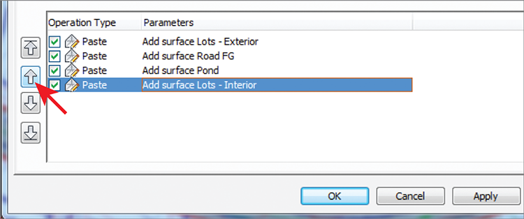
Figure 18-3: Clicking the up arrow changes the order of operations so that the Lots – Interior surface is pasted before the Pond surface.
Repeat steps 7 and 8, this time selecting the Lot Daylight surface.
Contours are now shown in the area between lots 73 and 76, and all design grading for the project is represented as one surface (see Figure 18-4).
Save and close the drawing.

You can view the results of successfully completing this exercise by opening Combining Surfaces - Complete.dwg.

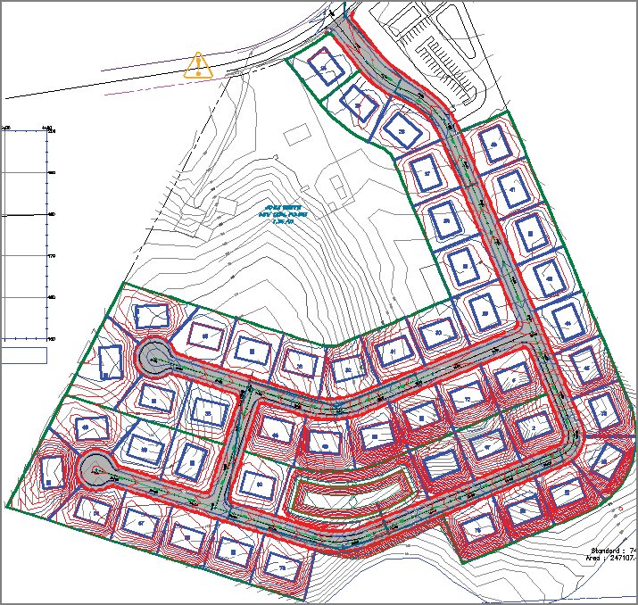
c18f004.tif — **Figure 18-4:** Grading for the entire project is represented by one surface.

Modular Design

In the preceding exercise, you saw five design surfaces listed in Prospector, each representing its own mini-design. The origin of these surfaces is as follows:

Lots - Exterior This surface is created from the feature lines used to grade all the lots except those enclosed between Jordan Court, Madison Lane, and Logan Court. The feature lines were added to the Lots - Exterior surface as breaklines. A polyline was drawn along the back edges of the lots and added to the surface as an outer boundary. The surface was allowed to triangulate across the road and interior lot areas. The following image shows the Lots - Exterior surface in 3D.

Lots - Interior This surface is created from the feature lines used to grade all the lots enclosed between Jordan Court, Madison Lane, and Logan Court. The feature lines were added to the surface as breaklines. A polyline was drawn along the front edges of the lots and added to the surface as an outer boundary. The surface was allowed to triangulate across the pond area. The following image shows the Lots - Interior surface in 3D.
Pond This surface is created from the grading group used to design the pond south of lots 69 and 70. The following image shows the Pond surface in 3D.
Road FG This surface is created from the road corridor. The following image shows the Road FG surface in 3D view.

Lot Daylight This surface is created from a grading group used to design the daylighting between lots 73 and 76. It’s shown in the following graphic in red along with the Road FG surface and Lot - Exterior surface in tan.

In the preceding exercise, you combined all these surfaces to create a single finished ground surface, as shown in 3D view in the following image.

Analyzing Design Surfaces

You can do many more things with a Civil 3D surface than just display contours. Unfortunately, I can’t discuss them all in a single chapter, let alone a section in a chapter; but I will cover several of the most commonly used surface-analysis features available in Civil 3D. I’ve grouped these features into three categories: surface analysis, hydrology tools, and quick profiles.

Using Surface Analysis

In the context of this category, surface analysis refers to the functions that appear on the Analysis tab of the Surface Properties dialog box. Here you can perform detailed analyses relating to elevations, slopes, contours, and watersheds (see Figure 18-5). The results of an analysis are shown graphically in the drawing and, depending on the type of analysis, can appear as shaded areas, arrows, contours lines, or even 3D areas—all color-coded for the identification of different ranges of data. In addition, you can create a legend to help convey the meaning of each color.

Performing an analysis can be thought of as a two-step process. The first step is to create the analysis ranges in the Surface Properties dialog box. This step doesn’t produce anything visible in the drawing, but it creates the data that will be used to generate graphical output. To create something visible in the drawing, you must perform the second step, which is to assign a style to the surface that displays the components of that analysis. For example, to display the slope arrows for a surface, you must first create the slope ranges and then apply a surface style that has slope arrow display turned on.

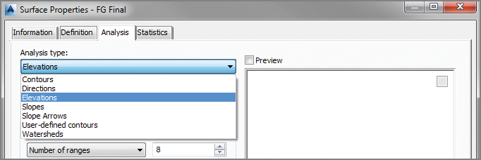
c18f005.tif — **Figure 18-5:** The Analysis Type choices available on the Analysis tab of the Surface Properties dialog box

Exercise 18.2: Analyze Surfaces

In this exercise, you’ll perform a slope analysis to identify steep-slope areas in the project. You’ll then adjust one of the lots to demonstrate how an analysis can be used as a design tool.

Open the drawing named Analyzing Surfaces.dwg located in the Chapter 18 class data folder.

This drawing contains the FG Final surface that you created in the previous exercise.
Click one of the red or blue contours in the drawing, and then click Surface Properties on the ribbon.
On the Surface Properties dialog, on the Analysis tab, select Slopes as the analysis type. Under Ranges, enter a value of 4 in the Number field.
Click the Run Analysis icon (downward-pointing arrow).
Four ranges are listed in the Range Details section of the dialog box.
Edit the slope ranges as follows:

For ID 3, you must enter the Maximum Slope value first and then the Minimum Slope value.

IDMinimum SlopeMaximum SlopeColors10.0000%2.0000%222.0000%10.0000%3310.0000%34.0000%30434.0000%1158.7766%1

Click the Information tab, and change the style to Slope Banding (2D). Click OK, and then press Esc to clear the selection of the surface.

The red areas are of particular concern because they represent slopes that aren’t stable with the type of soil found on this site.

As shown in Figure 18-6, the drawing displays colored areas indicating excessively flat slopes (0%–2%) in yellow, moderate slopes (2%–10%) in green, steep slopes (10%–34%) in orange, and excessively steep slopes (>34%) in red.

Figure 18-6 Colored areas indicate different slope ranges in the FG Final surface.
Click one of the colored areas to select the surface, and then right-click and select Display Order ⇒ Send To Back.

This displays the feature lines and other drawing graphics on top of the colored shading rather than hidden beneath it.

More about Slopes

Slopes are a significant aspect of land development design. For every project, certain slope ranges are targeted for specific purposes. These ranges can vary from project to project.

For the example project, you’re interested in knowing where there are excessively flat areas (yellow, 0%–2%), because those areas could potentially have drainage problems. Yellow areas on building pads are OK because there will be buildings in those locations; but yellow areas on roads could represent drainage issues.

Green areas (2%–10%) represent slopes that can be traveled safely on foot or with a vehicle. You want the entire road surface to be green, and there should be enough area between each building pad and the street to install a driveway.

Orange areas (10%–34%) represent places where travel isn’t possible but where the slopes are still stable and safe from collapse. In this project, you would expect the pond embankments and the backs of some of the lots to be orange. Orange areas on the road and entire front yards that are orange aren’t acceptable.

Finally, red areas represent slopes that are too steep for the soil to support. These areas would be subject to collapse and are considered dangerous. Red areas must be removed.

Press Esc to clear the previous selection. In the upper-right viewport, click the blue rectangular feature line at the center of lot 70. On the Edit Elevations panel of the ribbon, click Raise/Lower.

If the Edit Elevations panel isn’t visible, click Edit Elevations.
When you’re prompted on the command line to specify an elevation difference, type -5 (-1.524) and press Enter.

You may need to redo steps 2–6 to reestablish the ranges and colors.

After a pause, the surface rebuilds, and the red area in lot 70 is removed. The front yard is still green, which means it’s in the slope range to install a driveway (see Figure 18-7).
Save and close the drawing.

You can view the results of successfully completing this exercise by opening Analyzing Surfaces - Complete.dwg.

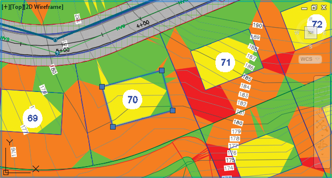
c18f007.tif — **Figure 18-7:** Lot 70 after the building pad has been adjusted downward to eliminate the steep slope

Using Hydrology Tools

Civil 3D provides two very useful tools to help you analyze the drainage performance of your surface: Water Drop and Catchments. The Water Drop tool shows you the theoretical path of a drop of rain as it flows downhill from a location you specify. By analyzing this path, you can determine the direction of flow and find low spots where water will stop flowing and begin to accumulate. A catchment shows you the area that drains to a point you specify. This is helpful for stormwater-management design, such as determining how large an inlet opening needs to be based on the size of the area contributing runoff to it.

Exercise 18.3: Analyze Hydrology

In this exercise, you’ll use the Water Drop tool to analyze the flow of runoff to two inlets. Then you’ll use one of the Catchment tools to determine the area contributing runoff to that inlet.

Open the drawing named Using Hydrology Tools.dwg located in the Chapter 18 class data folder.

In this drawing, the feature-line layers have been turned off. Also, a new surface named EG-FG Composite has been provided. This surface was made by creating a new surface and pasting EG and FG Final into it. The purpose of this surface is to enable the analysis of the entire project as though it has already been built.
Click the Analyze tab of the ribbon, and then click Flow Paths ⇒ Water Drop.
When prompted to select a surface, press Enter to indicate that you would like to select the surface from a list.
On the Select A Surface dialog, click EG-FG Composite, and then click OK.
On the Water Drop dialog, click OK to close the Water Drop dialog box.
In the left viewport, click a point in lot 29 near the road. A blue water-drop path is drawn from lot 29, down the curb line, to the inlet near station 2+50 (0+080). You can see the path in the lower-right 3D viewport as well.
With the Select point: prompt still active, click a point near the southeast corner of lot 23.

This water-drop path travels toward the west along the curb line of Madison Lane. It ends at the inlet near station 7+25 (0+220) on Madison Lane.
Press Esc to clear the current command. On the Analyze tab of the ribbon, click Catchments ⇒ Create Catchment From Surface.
When prompted to specify a discharge point, in the left viewport, use the Center object snap to choose the center of the red circle at the end of the second water-drop path you created.
On the Create Catchment From Surface dialog, select EG-FG Composite for Surface, and click OK.

Catchments are visible only in plan view, so you don’t see the catchment in the lower-right model view.

A blue outline indicates the shape of the catchment area that drains to the inlet at the location you selected.
Save and close the drawing.

You can view the results of successfully completing this exercise by opening Using Hydrology Tools - Complete.dwg.

Using a Quick Profile

In Chapter 7, “Designing Vertically Using Profiles,” you learned how to create surface profiles using alignments and surfaces. You also learned that a profile is a useful tool that enables you to slice through your design and view it from a different perspective. Well, what if you could create a profile from a whole list of entities that are readily available in your drawing? You can, and the command that does it is called Quick Profile.

The Quick Profile command creates a temporary profile along the path of a line, an arc, a polyline, a parcel line, a feature line, a survey figure, or a selected series of points. Once you have selected the object to represent the path, you’re presented with a dialog box that enables you to select any surface in the drawing that you would like to display in the temporary profile view. If you have selected a 3D object such as a 3D polyline or feature line, you’re also given the option to represent that object as a profile.

If you modify the object you used to define the path of the profile, the quick profile view updates automatically. This is a great tool for viewing slices of your design at many different locations very efficiently. Quick profiles are intended to be temporary, and they disappear whenever you save the drawing.

Exercise 18.4: Analyze Using a Quick Profile

In this exercise, you’ll use quick profiles to study the interaction between existing ground and proposed ground in the pond area and in the area between the interior lots.

Open the drawing named Using a Quick Profile.dwg located in the Chapter 18 class data folder.
In this drawing, a heavy red polyline in the left viewport crosses through the entire project at the location of the pond.
Click the Analyze tab of the ribbon, and then click Quick Profile.
When you’re prompted to select an object, click the heavy red polyline that crosses through the pond.
On the Create Quick Profiles dialog, verify that the box next to Select All Surfaces is unchecked; then check the boxes next to EG and FG Final. Select Design Profile as the profile style for FG Final.
Click OK, and then click a point in the lower-left corner of the upper-right viewport.
A new profile view shows existing ground in red and proposed ground in black. As you study the profile, you should be able to identify the shape of the road in two locations and the shape of the pond in between (see Figure 18-8).

Figure 18-8: Several prominent design features can be noted in the quick profile.
Click the red polyline to show its grips, and then click one of the grips and move it to a new location.

Notice the change to the quick profile. Use the red polyline and the quick profile to study the design of the project at several different locations.
Press Esc to clear the selection of the red polyline. Zoom in to the interior lots, and identify the green feature line that forms the back sides of lots 68–70.
Click Quick Profile on the ribbon. When you’re prompted to select an object, click the green feature line described in the previous step.
On the Create Quick Profiles dialog, check the box next to EG. Make sure the Draw 3D Entity Profile option is checked, and then select Design Profile as the 3D Entity Profile Style.
Click OK, and then click a point to the right of the first profile view.

The 3D Entity options weren’t available the first time you used the Quick Profile command because the red polyline you selected was a 2D object.

A new profile view is created that shows existing ground in red and a profile of the feature line in black. Notice how the feature line matches existing ground except for a certain length at either end where it ties into the finished ground elevations (see Figure 18-9).

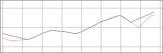
Figure 18-9: A quick profile view showing a feature line and a surface profile
Save and close the drawing.

You can view the results of successfully completing this exercise by opening Using a Quick Profile - Complete.dwg. Note that the “Complete” version of the file isn’t much different from the original, because quick profiles are removed when the drawing is saved.

Calculating Earthwork Volumes

Moving earth is one of the most expensive construction activities in a land development project. For this reason, there are two important questions you’ll need to answer about nearly every grading design you do:

How much earth must be moved?
How much earth must be brought to or transported away from the project site?

As a designer or an engineer, one of your most important tasks is to answer these questions with the smallest values possible. The less soil that is required to be moved for a project, the more money you save the client and/or owner. Transporting soil to or from the site is also a very costly construction activity, so it’s also one you should minimize.

Understanding Earthwork Volumes

When talking about earthmoving, you’ll often use the terms cut and fill. Cut is soil material that is removed from the ground, and fill is soil material that is added to it. When an excavator takes a scoop of soil out of the ground, that soil is called cut. When that scoop is carried to another location on the site and dumped, the soil becomes fill. Grading the site is nothing more than a complex series of scoops and dumps—that is, cuts and fills. At the end of the project, all the scoops added together represent the cut value, and all the dumps added together represent the fill value. If these values are equal, then no soil needs to be transported to or from the site, thus reducing the cost of construction (not to mention the environmental impact). When cut and fill are equal, the condition is referred to as a balanced site. As a designer, you should strive to balance the earthwork of your designs whenever possible.

Using the Volumes Dashboard

Although you can use several methods to calculate earthwork volumes in Civil 3D, I’ll cover only one of them in this book in detail: the Volumes Dashboard. The Volumes Dashboard command is found on the Analyze tab of the ribbon. Clicking this opens Panorama, which displays the Volumes Dashboard tab. Here, you can add or create one or more TIN volume surfaces, and the cut and fill results are shown. You can also create bounded volumes, which are smaller areas within a volume surface that might represent individual lots or project phases. You can even generate detailed reports that are displayed in a browser or in Civil 3D, as shown in Figure 18-10.

Exercise 18.5: Analyze Earthwork

In this exercise, you’ll use the Volumes Dashboard to analyze the cut and fill for the entire project as well as three individual lots.

Open the drawing named Calculating Volumes.dwg located in the Chapter 18 class data folder.
Click the Analyze tab of the ribbon, and then click Volumes Dashboard.

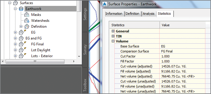
Figure 18-10: A TIN volume surface named Earthwork shown in Prospector, and its volume results shown in the Surface Properties dialog box
On the Volumes Dashboard tab of Panorama, click Create New Volume Surface. In the Create Volume Surface dialog box, do the following:
1. For Name, enter Earthwork.
2. For Style, select _No Display.
3. For Base Surface, select EG.
4. For Comparison Surface, select FG Final.
5. Click OK.
  
  What’s a TIN Volume Surface?
  
  As you may recall from Chapter 4, “Modeling the Existing Terrain Using Surfaces,” the acronym TIN stands for Triangular Irregular Network, which is a method of creating surfaces by drawing lines between 3D points to form triangles. A TIN surface is any surface that is created using this method. When you create a TIN volume surface, Civil 3D superimposes one TIN surface over another and creates a point at each location where the triangle edges cross. New triangles are then created by connecting the calculated points. The resulting surface has the same distinctive triangular shapes, but instead of elevations, the values it represents are differences in elevation between the two surfaces. These differences in elevation are referred to as cut when they are negative and fill when they are positive.
The cut and fill results are shown in Panorama. Here, you see that the Cut Volume value is much smaller than the Fill Volume value. The project isn’t balanced, and the requirement for extra fill means soil will have to be delivered to the project site. The design should be adjusted to bring it closer to balance. This can be accomplished by lowering the profiles and building pad feature lines to create more cut while eliminating the need for fill.
Click Earthwork, and then click Add Bounded Volume. When you’re prompted to select Bounding Object, click the parcel area label of lot 1.
Repeat the previous step for lots 2 and 3. Click the plus sign next to Earthwork to expand the information below it.

Note the individual cut and fill results that are shown for lots 1, 2, and 3.
Other Volume Methods

Civil 3D provides three additional methods for calculating cut and fill:
1. TIN Volume Surface You can create a TIN volume surface without using the Volumes Dashboard by simply using the Create Surface command and choosing TIN Volume Surface as the type. You can view the volume results for the surface by opening Surface Properties and clicking the Statistics tab.
2. Grading Volume Tools You use the Grading Volume Tools with grading groups that have been assigned a volume base surface. Not only can the Grading Volume Tools report cut and fill, but they can also be used to adjust the design and even balance the design automatically.
3. Quantity Takeoff Criteria You use Quantity Takeoff Criteria to generate section-by-section volume calculations based on a sample line group. This method is nearly always associated with a corridor model for a transportation design project.
Checking the boxes tells the Volume Dashboard to include information for these items in the report.

Change the name of Earthwork.1 to Lot 1, Earthwork.2 to Lot 2, and Earthwork.3 to Lot 3. Check the boxes next to Lots 1, 2, and 3, and then click Generate Cut/Fill Report.
Your browser should open, displaying a detailed cut-and-fill report for the overall earthwork as well as the three individual lots.
Save and close the drawing.

You can view the results of successfully completing this exercise by opening Calculating Volumes - Complete.dwg. Although there is no change to the drawing itself, you can open the Volumes Dashboard and view the volume calculations.

Labeling Design Surfaces

As you have done with every other type of design in this book, you need to annotate your surface design. Like all annotation, the information you convey here is almost as important as the design itself, particularly with regard to grading.

From a strictly documentation standpoint, the primary final product of a grading design is a set of design contours. By themselves, the contours aren’t very useful for construction. Once they are labeled, however, they begin to show the contractor exactly how to shape the land to meet its desired function. In some areas, contours alone don’t provide enough detail and must be supplemented with labels that call out specific elevations and slopes. Labels that refer to the elevation of a single point on a drawing are often referred to as spot elevations or spot grades.

Although it was some time ago, you learned how to create contour, spot, and slope labels in Chapter 4. You’ll apply those skills once again, but this time you’ll label proposed elevations rather than existing elevations.

Exercise 18.6: Label a Design Surface

In this exercise, you’ll create contour, spot elevation, and slope labels for lot 2. You’ll use these labels to adjust the design of lot 2.

Open the drawing named Labeling Design Surfaces.dwg located in the Chapter 18 class data folder.

The upper-right viewport is zoomed in to the first few lots at the beginning of Jordan Court. You’ll add labels in this area to provide information about contour elevations, slopes, and spot elevations.
Click the Annotate tab of the ribbon, and then click Add Labels.
In the Add Labels dialog box, do the following:
1. For Feature, select Surface.
2. For Label Type, select Contour – Multiple.
3. Click Add.
When you’re prompted to select a surface, click one of the red or blue contours in the drawing.
When prompted to specify the first point, pick two points that draw a line through the contours in the front yard of lot 2 (see Figure 18-11).
In the Add Labels dialog box, change Label Type to Contour – Single. Click Add.
When you’re prompted to select a surface, click one of the red or blue contours in the drawing.
Click several contours on the Jordan Court road surface.

Figure 18-11: Contour labels in the front yard of lot 2
In the Add Labels dialog box, change the label type to Slope. Click Add.
When prompted to select a surface, click one of the red or blue contours in the drawing to select the surface.
When prompted to choose between the One-Point and Two-Point labeling options, press Enter to select the One-Point option. Pick a point near the center of the front yard of lot 2.
The slope label indicates that the grade here is greater than the allowable 10%. This is something you’ll address at the end of this exercise.
In the Add Labels dialog box, change the label type to Spot Elevation.
Click Add, and select a red or blue contour when you’re prompted to select a surface.
Using an Endpoint object snap, select the four corners of the lot 2 building pad. This places a spot-elevation label at each corner.

Press Esc to clear the previous command. Click the blue building pad feature line for lot 2. On the Edit Elevations panel of the ribbon, click Raise/Lower.

If the Edit Elevations panel isn’t visible, click Edit Elevations.
When you’re prompted to specify the elevation difference, type -2 (-0.691) and press Enter.
After a pause while the software rebuilds the surface, the contour labels, slope label, and spot-elevation labels all update to reflect the change (see Figure 18-12). The slope in the front yard of lot 2 is now less than the maximum of 10%.
Save and close the drawing.

You can view the results of successfully completing this exercise by opening Labeling Design Surfaces - Complete.dwg.

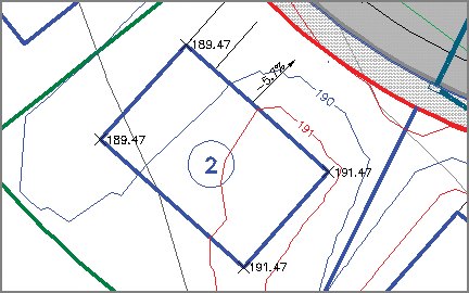
c18f012.tif — **Figure 18-12:** The labels update, indicating that the maximum slope requirement is now met for lot 2.