
Chapter 4
Defining a Highly Available Messaging Solution
As you saw in Chapter 1, “Business, Functional, and Technical Requirements,” when eliciting requirements, desired availability is often one of the first topics to be raised. It is important to note that one of your functions as a consultant or implementer is to make the businesses aware that raising the availability of any system has a direct cost implication.
With quality cloud-based solutions, messaging systems are no longer shackled to the limits of on-premises capabilities. Keep cloud-based solutions in mind as a possible fit for some of your highly available messaging solution requirements.
If you have deployed Exchange Online in conjunction with on-premise solutions, and you are running in Hybrid mode, then you need to consider how the Exchange Online service-level agreement dovetails with your on-premise service-level agreement. In traditional on-premise systems, the more available a system becomes, the more expensive it is to operate. The price of increasing availability, however, is often offset by the cost of an outage. For a large company or well-known brand, an email outage may become a visible public failure with an associated loss of confidence.
The definition of availability and how that availability is measured is one of the key factors in the choice of technology you will use to implement in your design. One of the critical factors to establish is how the availability of the system will be measured and what the context for that measurement will be. We will use the following formula to calculate availability levels:
percentage availability = (total elapsed time – sum of downtime)/total elapsed time
Using the example of 99.9 percent availability, which is often noted as “three nines” availability, this translates to the system suffering downtime of 8.76 hours on an annual basis. That may not sound like a lot; if the measure is changed to three nines per day, this translates to 1.44 minutes of downtime, which may or may not be enough time for a reboot to occur.
If you calculate the permutations from one nine to five nines, you will understand why you don't often hear of systems that are available beyond five nines, as shown in from Table 4.1. This depends, however, entirely on how the availability is measured.
Table 4.1 Availability by the nines
One of the many things you'll do during requirement elicitation is to help the business define and understand the services that Exchange delivers in terms of Exchange availability. At minimum, Exchange availability is a superset of dependency services. These services may be classified as follows:
For the sake of clarity, we will not define auxiliary services such as message hygiene third-party application integration, or the many other examples that come to mind. Assuming you are satisfied to continue with the three basic services listed, your criteria may also include that availability could be measured per service. The availability of a system consisting of several independent critical components is a product of the availabilities of each individual component. The product is calculated by multiplying together the availabilities of each individual component in the following manner:
A(n) = A1 × A2 × … × An
In the case of three components, our equation becomes
A(3) = A1 × A2 × A3
Let us examine a hypothetical example of three nines availability across three hypothetical components, as shown in Table 4.2. Using Excel, you would list the three availability components and use the PRODUCT function to multiply the three numbers together. Or, you could simply multiply the first number by the second number and then by the third number to obtain the fourth number, or result. Since we have multiplied three numbers together to obtain a fourth number, we need to move our decimal to the left by four places, or divide by 10,000 (four zeroes), to obtain a number that may be expressed as a percentage availability. The result will look similar to Table 4.2.
Table 4.2 Component availability
| Component | Percent Availability |
| Client access | 99.9 |
| Email transport | 99.9 |
| Email storage | 99.9 |
| Total availability | 99.7 |
Notice that the total availability is lower than the availability of any of the component pieces. In order to build a system with a particular stated resilience, the components' availability requires examination. This may include network, power, chassis, and storage availability to name just a few, because these are all dependent features in larger systems.
Figure 4.1 illustrates the interdependency of component systems. Note that each one of the boxes of components can carry its own availability measurement when calculating total system availability.
Figure 4.1 clearly illustrates that it is extremely difficult to establish even theoretical total system availability when so many systems are interrelated. When agreeing on the resulting availability of the desired system, clarify the definition of availability, downtime, and scheduled downtime as it pertains to the business.
Scheduled system downtime classically is not included in how availability is measured—in our three nines example, 1.44 minutes per day does not allow for much action to be taken. However, if the measure is adjusted to per year, then 8.76 hours becomes much more plausible for system maintenance.
Defining the cost of downtime may appear to be an emotional measure, and it may seem somewhat intangible. In this section, we will look at turning some of the intangibles back into definable measures.
Often the actual cost of downtime may be difficult to measure without an understanding of the business in question and how the services provided by Exchange fit into the processes deemed mission critical. We will examine a number of examples of businesses in different vertical markets:
Each of these businesses has a critical path enabled by email and an average cost or value associated with it. For example, if an average day's worth of transactions is $500,000, and this amount represents 1,000 transactions, the average transaction value is easily calculated as $500. The financial transaction may have multiple email interactions associated with it, so there is little point in trying to calculate the average cost of an email. If the bulk of the transactions are occurring over a 10-hour period, and assuming that customers' transactions occur evenly throughout the day, then each hour's transactions may be worth $50,000.
Continuing with our example, assuming a two-hour outage during which email-based transactions cannot occur, the business may face a loss of at least $100,000. Very often, however, this represents only the tip of the iceberg in terms of financial losses, because the damage to the business's reputation may multiply this number in terms of transactions that will not occur in the future. That is, customers may elect to move their business to another company that they deem is more reliable. This is particularly prevalent in the retail, online, and premium brand segments.
If email is part of the critical transaction path, then the hourly cost of the workers who are attempting to facilitate the transaction, as well as in-house or third-party personnel who are endeavoring to rectify the failure, are added to the cost of the downtime. With this in mind, we are able to measure in part some of the more tangible losses accrued to downtime. We say “in part” because reputational and confidence losses may cascade for months or even years to come. In the following equation, we include the percentage impact, since rarely is the outage 100 percent, with the exception of an actual disaster, of course.
lost revenue = (gross revenue/business hours) × percentage impact × hours of outage
cost of the outage = personnel costs + lost revenue + new equipment
From these equations, we are able to compute a value. It is worth restating, however, that this value may represent only a portion of the total attributable loss due to confidence and reputational loss.
A bank may argue that email is a non-mission-critical system, since the equipment and software required to process transactions during the day are represented via mainframes and traditional banking systems. Nonetheless, confidence loss comes into play here as well. Since email is ubiquitous, no bank is immune from the confidence loss, which may occur if its customers or partners are unable to email for two or three days at a time. This time frame is quite realistic when faced with even a small outage without redundancy in place.
Failure of systems or components is inevitable. However, you will be better able to plan for failure as you come to understand that failure is not a random event by which to be taken by surprise. Rather, it should be a carefully planned scenario. We will use drives as our topic for discussion of failure, because there will be more drives in your deployment than there are servers, racks, or cooling units. Nevertheless, the logic presented here applies equally to all of these components.
Hardware components have a published annual failure rate (AFR), which is simply the rate at which the component is expected to fail. One hundred SATA drives assembled in a system will suffer an approximate failure rate of 5 percent. Does that mean that for every 100 drives, we need to keep 5 spares available on a shelf? Not quite. It does, however, lead us down the road of planning for failure, as we consider factors such as database distribution within a database availability group (DAG) or how many servers to deploy in order to satisfy a services dependency.
Earlier, we defined total availability as the product of component availability. However, you will recall that the three components with an availability of 99.9 percent had a total availability of only 99.7 percent. A similar mathematical model is available when we add multiple components to a given system.
The logic used for calculating the probability of failure when using identical components is to take the probability of failure of the component and calculate to the power, as opposed to the product. The probability of failure of a system consisting of several identical redundant components is a product of the probabilities of failure of each component. Because all probabilities are identical, the product becomes a power:
P(n) = P × P × … × P = Pn
The difference between the availability and probability of failure is that in the first case, each component must be available in order for the entire system to be available, whereas in the second case, each component must fail in order for the entire system to fail. We will use probability of failure of identical SATA drives to demonstrate this principle.
Remembering that SATA drives have an expected failure rate of 5 percent, the first drive has a probability of failure of 5 percent, P1 = P = 5%. In other words, the probability of one drive failing (P1) is the same as the overall probability of failure (P1 = P), which we know is 5 percent, thus P1 = P = 5%.
Things become more interesting as soon as we add a second identical component into the same system. For two identical drives, we will use the notation of P2, three identical drives P3, and so on. Assuming up to four components in a system, you will note that the probability of failure drops considerably.
P1 = P = 5%
P2 = P2 = 0.25%
P3 = P3 = 0.0125%
P4 = P4 = 0.000625%
As the probability of failure becomes smaller, the availability value of the system increases. Availability (A) is calculated as An = 1 – Pn. Using our one-drive example, this becomes A1 = 1 – 5% = 95%. As we add multiple drives or identical components to a system, system availability increases radically:
A1 = 1 – 5% = 95%.
A2 = 1 – 0.25% = 99.75%
A3 = 1 – 0.0125% = 99.9875%
A4 = 1 – 0.000625% = 99.9994%
While we have used this logic to demonstrate failure rates with drives, we can also apply the identical logic to calculate the probability and possible availability of individual systems or system components such as switches, servers, datacenters, and so forth.
When thinking about Exchange 2013, however, the logic is even simpler. Two CAS servers per location are better than one, and four database copies on SATA drives have a probability of failure of 0.000625 percent and, reciprocally, an availability of 99.9994 percent.
Taking it as a given that failures are an event for which you must plan, you can look for and mitigate failure domains. Failure domains are service interdependencies or shared components of a system that are able to reduce the overall availability of the system, or they may introduce a significant impact to the overall system should a failure occur.
An obvious example of a failure domain in a datacenter is a single power source. Should that power source fail, then the entire datacenter fails. Similarly, we can think of power to a rack, shared-blade chassis, non-redundant switches, and cooling systems as other obvious examples. A not-so-obvious example might be a storage area network (SAN). SANs tend to be designed with redundancy in mind. However, as we observed when we calculated the probability of failure of a single component, it makes sense to use multiple database copies. The benefit of those multiple database copies is nonetheless negated if they are stored on the same SAN, because the probability of failure is now identical to that of the SAN itself, as opposed to a fraction of what it could be, even when choosing multiple, identical, cheap drives.
Virtualization introduces similar failure domains. If you elect to virtualize, then know that each host represents a failure domain. It makes sense to distribute your Exchange components over different hosts, as opposed to centralizing them onto a single host.
When planning for failure, isolation and separation are great concepts to use in your datacenters. Isolation of components—for example, using multiple cheap drives as opposed to shared storage—increases availability considerably. Separation significantly reduces the number of shared failure domains. When Exchange servers are distributed across multiple racks, servers, or even virtualization hosts, the probability of overall failure increases dramatically as the number of service interdependencies, or possible failure domains, decrease dramatically.
Well-publicized failures of public cloud-based services have taught us that as systems scale, complexity and interdependencies increase and failure becomes inevitable. Operational efficiency is a significant factor in maintaining availability. How you respond to a failure can significantly increase or decrease outage times.
Service-level agreement, recovery point objective, recovery time objective, high availability, and disaster recovery are common terms used when discussing availability. In this section, we will discuss each of these terms with regard to a messaging system, which is part of a larger IT ecosystem.
A service-level agreement (SLA) is an agreement between a business and an IT vendor, which defines the services that the IT vendor will deliver to the business, as well as the uptime, or availability, of each service. The SLA must include how availability will be measured. This could be a complex exercise, depending on the constituent pieces of each service. As an example, for which of the following is the Exchange storage tier considered available?
How SLAs are measured and reported is an important matter when documenting requirements. It is one of the items that you must clarify, turning assumptions into documented facts, using the skills you learned in Chapter 1.
Recovery point objective (RPO) and recovery time objective (RTO) factor strongly in SLA definitions. Figure 4.2 represents an example of a very simple system or non-highly-available server. It is worth starting with a simple example in order to baseline your understanding of these concepts. Just be aware that the example shown in Figure 4.2 is not representative of all the possible highly available configurations that are achievable using Exchange 2013.
High availability (HA) and disaster recovery (DR) are sometimes incorrectly used interchangeably when, in fact, they are quite different from each other. The one thing that they do have in common is that because of some level of duplication of hardware, software, networks, storage, or other components, the overall cost of the system goes up, commensurate with the level of redundancy required.
A high availability (HA) system is defined as a system that includes redundant components that increase the availability or fault tolerance of the overall system in a near-transparent manner and confined within a defined geography. It is also important to note that HA is a technology-driven function; that is, the technology used in making the system highly available is often the same one that initiates a failover to another available system or component of that system. In other words, IT is responsible as the initiator of the failover as well as being the decision maker to fail a system over.
Disaster recovery (DR) is defined as the restoration of an IT-based service. It includes the use of a separate site or geography, and it addresses the failure of an entire system or datacenter containing that system. It includes the use of people and processes to make DR possible. Lastly, DR is hardly ever seamless or swift.
Consider this example: Datacenter A houses multiple copies of data within a highly resilient cluster representing the implementation of an email service. Datacenter B has a single server with a near-identical specification as one of the servers in Datacenter A, except that it has a tape drive attached. If Datacenter A is lost, a restore of the last-known good backup will occur in Datacenter B—however long it takes. From that point forward, the single server in Datacenter B represents the restoration of the service that used to live in Datacenter A. There may be a significant gap in the data restored in Datacenter B, depending on when the outage occurred, as well as the point in time of the last known good backup. If no good backup can be found, then Datacenter B will offer a “dial tone” service for email, which means that customers may send and receive email. However, no historical mail, contacts, or calendar information will be present in their mailboxes. There is a sharp contrast between what was implemented in Datacenter A versus what was implemented in Datacenter B.
This kind of dramatic contrast between locations can be expected as companies figure out how to balance the cost of a DR facility with the stated RPO and RTO. The lower the RPO and RTO, the higher the cost of the overall solution.
As stated at the beginning of the chapter, raising the availability of any system has a direct cost implication. Exchange is in a league of its own in terms of interdependency with other systems, as illustrated in Figure 4.1. Following are a number of factors to consider that will dramatically influence both cost and complexity when planning for high availability:
This is not meant as an exhaustive list of all possible factors. Your own analysis of your environment may yield a number of other factors that may be relevant.
Once you identify the factors influencing availability, you can evaluate each in an attempt to mitigate them. For example, let's say your analysis has shown that cooling and the centralization of all IT into a single datacenter represent a single point of failure. The business will remedy the lack of cooling redundancy, but it will not build or rent another datacenter. You may want to capture this and other potential factors as demonstrated in Table 4.3.
Table 4.3 Availability factors and mitigation
| Factor | Detail | Mitigation |
| Datacenter | Only one datacenter exists currently, which makes it impossible to achieve the stated disaster recovery goals. | The customer has been advised of the risk and has chosen to not invest in another datacenter. The stated disaster recovery goals have been adjusted accordingly to reflect a longer time to recover. |
| Cooling | Two cooling units service the datacenter with insufficient individual capacity to assume the full cooling requirement in the event of failure. | The customer has elected to upgrade the cooling units. |
| Virtualization | The customer has deployed a virtualization solution on shared storage SAN, which automatically moves guests to the least-busy node. Customer wishes to deploy a DAG. | After reviewing the Exchange support statement and possible storage models, the customer has decided to deploy on physical hardware. |
| Network/mail flow | The customer has deployed a point solution for branding and hygiene in the DMZ. No redundancy exists. | The customer has elected to replace a point solution with a cloud-based equivalent. This equivalent presents an SLA with 99.99 percent availability. |
When calculating availability (remember that total availability is a product of all the availability factors), the biggest factor influencing total availability is the component(s) in the entire chain that is most likely to fail. As you saw in Table 4.2, when calculating total availability, a single machine is not very redundant, and it is able to drop the total availability of a single factor, such as networking or mail flow, quite significantly.
In order to tie the concepts in this chapter together, let us consider the concepts introduced here as well as the high-availability features built into Exchange that were presented in Chapter 3, “Exchange Architectural Concepts.”
When setting a high-availability goal, consider your recovery priorities; that is, do you want to recover quickly? Do you want to recover to the exact point of failure? Or do you want to do both? Also consider which services are critical and require a level(s) of redundancy or higher availability. Finally, you also need to decide which of the features introduced in Chapter 3 make sense in terms of your high-availability requirement versus those that are just nice to have.
The following sections examine major Exchange concepts or features in the light of high availability.
Transport is the superset of features and functions of the Hub Transport role, including the sending and receiving of messages via SMTP as well as the redundancy features included in Exchange 2013, such as shadow redundancy and shadow transport.
In Chapter 3, you learned that Safety Net is an improved version of the transport dumpster in Exchange 2010. Shadow redundancy was similarly introduced in Chapter 3. Due to the automation capabilities in Safety Net and shadow redundancy, very little else needs to be considered—except for the location of the transport queue. If you are planning for an outage of any sort that may cause email to queue or to be deferred, as in the case of Safety Net, make sure that you allocate enough storage on the volume containing the storage queues. Safety Net and shadow redundancy both transport lower RPO. Transport itself, however, may cause an outage if the queue location has not been taken into account.
During an outage, email queues may grow considerably. If Exchange is installed on the system volume, or the queues are not located on a dedicated volume, then an outage may be exacerbated considerably by a disk-full condition on an Exchange server.
Your availability concerns for transport will include:
Namespace planning is often a misunderstood topic. The impactions for high availability, however, are substantial. The cheaper side of misunderstanding this topic is an incorrect set of names on a Subject Alternate Name (SAN) certificate. The more expensive side is a total lack of system availability after a failover event has occurred.
As presented in Chapter 3, the minimum number of name spaces we need for Exchange 2013 has fallen to two. For example, using our Exchange-D3.com name space in a single datacenter scenario, we need the following:
A graphical representation of the minimum number of name spaces required including a single internet protocol name space is shown in Figure 4.3. The details of each protocol may be found in Table 4.4.
Figure 4.3 Single name space

Table 4.4 Name spaces and protocols—single name space
| Name | Protocol |
| Autodisover.Exchange-D3.com | Autodiscover |
| Mail.Exchange-D3.com | SMTP |
| Mail.Exchange-D3.com | Outlook Anywhere |
| Mail.Exchange-D3.com | EWS |
| Mail.Exchange-D3.com | EAS |
| Mail.Exchange-D3.com | OWA |
| Mail.Exchange-D3.com | ECP |
| Mail.Exchange-D3.com | POP/IMAP |
Similarly, if we use a global load balancer or even Round Robin DNS, we are able to utilize a single name space. Table 4.4 is still valid in this scenario, because two virtual IPs representing each datacenter are stored in the global load balancer and presented to the external client simultaneously. The client will then attempt to access each datacenter's IP address as shown in Figure 4.4.
Figure 4.4 Single name space with global load balancer

We could quite easily extrapolate this example out to three, four, or more datacenters within a single name space. However, this assumes that connectivity from any point around the globe is roughly equal and that connectivity between datacenters is high speed in order to guarantee a good user experience.
For both of these examples, our SAN certificate entries remain simple:
Assuming, however, that you would like to present a different name space for Exchange housed in different datacenters, as shown Figure 4.5, the entries on your SAN certificate would read as follows:
Figure 4.5 Single name space across two datacenters

Remember from Chapter 3 that endpoint URL names are not important, since the autodiscover service is responsible for servicing endpoints to any requesting client. This implies that the URL endpoints may be named anything at all, as long as there is a valid path for the client to bind to the autodiscover endpoint.
You may choose to forego SAN certificates altogether and choose to implement a wildcard certificate; however, you are still required to plan your name spaces and define these in DNS.
Availability concerns for name space planning include:
Exchange Online presents its own set of SLAs, and it is of interest to us in terms of its interactions with on-premises Exchange. Assuming that your organization is running in Hybrid mode, there will be three on-premises points of interaction with Exchange Online. Specifically, these interaction points are as follows:
Each of these is not highly available by default because each is deployed on a single server. The only possible exception for keeping a single server may be directory synchronization, since it is built as a no-touch software appliance by default, unless deployed using the full-featured Forefront Identity Manager using a highly available SQL instance.
Exchange Client Access Servers providing Exchange Hybrid mode integration may be a subset of the total number of Client Access Servers contained in your organization. If more than one of these exists, they will be load-balanced via some sort of load-balancing mechanism. Client Access Servers facilitating Exchange Hybrid mode are responsible for the interaction between Exchange Online and on-premises Exchange and directly facilitate the features required, which makes the on-premises system and Office 365 appear as a single organization. With this in mind, you will do well to ensure that sufficient redundancy exists to guarantee availability during a server outage, as well as during periods of high server load.
Active Directory Federation Services (AFDS) enable external authentication to an on-premises Active Directory by validating credentials against Active Directory and returning a token that is consumed by Office 365, thereby facilitating one set of Active Directory credentials to be used against both on-premises services as well as Office 365. ADFS servers may have a DMZ-based component (ADFS Proxy servers) alongside the LAN-based ADFS server. ADFS Proxy servers are a version of ADFS that is specifically designed to be deployed in the DMZ, a secure network location, disconnected from a production network via additional layers of firewalls. Since all that these Proxy servers do is to intercept credentials securely and pass them onto LAN-based ADFS instances, they may not be required if an equivalent service is available via Microsoft TMG/UAG or similar.
These types of servers are great virtualization targets because of their light load. Depending on load, you will require a minimum of two ADFS servers and two ADFS Proxy servers.
Your availability concerns for Exchange Online/Hybrid mode include the following:
Database availability group (DAG) planning requires you to balance a number of factors. Most of these are interdependent and require significant thought and planning.
The theoretical maximum database size should not be based purely on the maximum database size supported by Exchange 2013. Large databases require longer backup/restore and reseed times, especially when over the 1 TB mark. Databases size of 1 TB and upward are impractical to back up, and they should only be considered if enough database copies exist in order not to require a traditional backup, specifically three or more copies. You need to strike a balance between fewer nodes and larger databases versus more nodes and smaller databases.
The number of database copies required in order to meet availability targets is a relatively simple determination. Early on, we discussed the number of disks or databases required in order to calculate a specific availability. If we have been given a stated availability target of 99.99 percent, then we will not be able to achieve such a target with a single database copy. Four copies within a datacenter is the minimum number required for a 99.99 percent availability target. Taking into account the number of databases is just one of the factors in our availability calculation.
In multi-datacenter scenarios, datacenter activation is a manual step, as opposed to the automatic failover provided by high availability. Therefore, switchover requires more time and incurs more downtime that an automatic failover. While Exchange 2013 is able to automate a switchover event, we would argue that the business via the administrator initiating the event should wield that level of control, so that the state of Exchange is always known and understood.
When the second datacenter uses RAID to protect volumes on a single server, as opposed to individual servers with isolated storage, this slightly increases the availability of each individual volume and therefore slightly increases overall availability. In the case of three or more database copies, however, the additional gain will hardly justify the additional costs of doubling the disk spindles (depending on the RAID model) and the additional RAID controllers. Applying the principle of failure domains, it may be cheaper to deploy extra servers with isolated storage, as opposed to deploying the extra disks and RAID controller per RAID volume required to achieve higher availability.
The number of DAG nodes is driven not only by the number of copies required but also by how many nodes are required in a database availability group in order to maintain quorum. Quorum is the number of votes required to establish if the cluster has enough votes to stay up or to make a voting decision, such as mounting databases. Quorum is calculated as the number of nodes/2 + 1. A three-node cluster can therefore suffer a single failure and still maintain quorum. Odd-numbered node sets easily maintain this mathematical relationship; however, even-numbered node sets require the addition of a file share witness.
The file share witness is an empty file share on a nominated server that acts as an extra vote to establish cluster quorum. Whichever datacenter in which the file share witness is located may be considered the primary datacenter. In Exchange 2013, the file share witness may be located in a third datacenter from the primary and secondary location, thereby eliminating the risk of split brain, which is a condition that occurs when two datacenters become active for the same database copy. Changes are now written to different instances of the same database, which requires considerable effort to undo should the WAN link between the primary and secondary datacentre break. This change, while not recommended, is now supported in Exchange 2013, and it is the first version of Exchange to support the separation of the file share witness into a third datacenter.
The distribution of databases on database availability group nodes has a direct impact on performance and availability. In order to demonstrate this concept, consider a four-node DAG with four database copies and with all databases active on Server 1, as shown in Figure 4.6.
Figure 4.6 Uneven database distribution
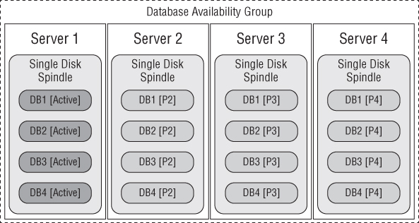
Server 1 will serve all of the required client interactions, while Servers 2, 3, and 4 remain idle, with the exception of logging replay activity. Assuming Server 1 fails, all active copies fail with the server and, depending on the health of the remaining copies, may all activate on Server 2. This is a highly inefficient distribution structure.
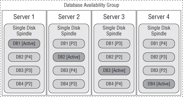
Figure 4.7 shows how databases are distributed in a manner such that client and server load is balanced and failure domains are minimized (assuming the storage is not shared). Note that this symmetry is precalculated on a current version of the Exchange calculator.
Figure 4.7 Balanced database distribution
In Chapter 3, we discussed how quorum is established and how Database Activation Coordination (DAC) mode affects DAG uptime. Remember that if you have DAC mode enabled on your DAG and a WAN failure occurs, both datacenters will dismount databases in order to prevent split brain. By design, DAC mode may be the cause of an outage if it is not implemented correctly. If properly implemented, however, it will act as an extra layer of quorum against split brain.
If WAN links are unreliable, and your DAG appears similar to Figure 4.8, consider planning your DAGs without DAC mode, as per Figure 4.9.
Figure 4.8 Single DAG with DAC mode

Figure 4.9 Multiple DAGs without DAC mode
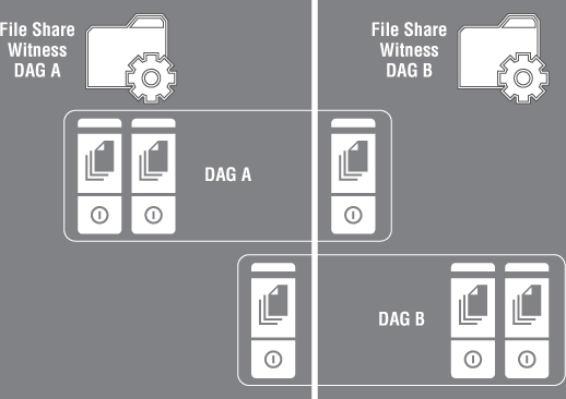
DAGs may be split into two or more DAGs with either datacenter maintaining quorum if a WAN failure occurs, similar to what appears in Figure 4.9.
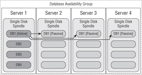
The bandwidth required for intersite replication may be considerable. Let's consider an example of a four-node DAG, with the first node containing all database copies, as shown in Figure 4.10.
Figure 4.10 DB1 before seeding

As the first database copy is added, we have a replication unit of traffic, as shown in Figure 4.11.
Figure 4.11 DB1 with one copy

As copies 3 and 4 are added, we have a multiple of this traffic, that is, replication traffic × 3, as shown in Figure 4.12.
Figure 4.12 DB1 with three copies
Exchange 2013 database replication is quite similar to that of Exchange 2010 in that it uses a single source as its replication master. Note that we are able to seed from any active or passive node in the DAG. This means that Server 3 can seed from Server 2. Likewise, Server 4 can seed from Server 3, all while Server 1 contains the active copy. If Server 3 and Server 4 are in different datacenters, then the replication traffic for all databases may outweigh the cost of placing two additional servers in the DR site.
Database sizing is critical, because reseed times are directly related to database sizes, especially if reseeds occur via WAN connections.
Assuming that you have established the AFR for your disks at 5 percent, you now have a potential number of reseed events that require planning. In Chapter 6, we will also discuss the automatic reseed capability of Exchange 2013. This capability is based on the forethought and planning required to ensure that the additional disks or LUNs have been allocated to each server so that Exchange may execute the automatic reseed.
Reseed times vary greatly across different networks. Therefore, it is vital to benchmark the time required to reseed a database under different conditions, because the reseed time factors directly into RPO and RTO times. Note that disks that are allocated as spares for automatic reseed targets suffer the same rate of failure as live production disks.
Your availability concerns for database availability group planning include the following:
There is no single way to achieve high availability. However, after working through the first few chapters in this book and armed with a set of requirements, you'll be able to build an availability model based on a solid set of requirements and the methodology needed to defend your design choices.

