Chapter 6
Univariable Analysis of a Nominal Dependent Variable

1. 6.1 Chapter Summary
2. 6.2 Glossary
3. 6.3 Equations
4. 6.4 Examples
5. 6.5 Exercises

Chapter Summary

Nominal data can be summarized by probabilities or by rates. Two special types of probabilities we encounter in health research are prevalence and risk. Prevalence of a disease is the probability that an individual chosen at random from a population will have that particular disease. Risk is the probability that a disease-free individual in the population will develop the disease during a specified period of time.

Rates are different from probabilities in that rates contain a measure of time in their denominator. The most commonly used rate in health research is the incidence of disease. Incidence is the number of cases of disease that develop per unit of person-time (e.g., per person-year).

Estimates of probabilities and rates do not come from Gaussian distributions. Instead, they come from either binomial (for probabilities) or Poisson (for rates) distributions. Interval estimation and hypothesis testing for probabilities and rates are usually accomplished using a normal approximation. A normal approximation means that the distribution of estimates is close to a Gaussian distribution. The justification for using a Gaussian distribution for interval estimation and hypothesis testing on probabilities and rates is that, like means of continuous data, estimates of probabilities and rates from all possible samples tend to come from binomial or Poisson distributions similar to a Gaussian distribution, especially when the sample's sizes are large (this is an application of the central limit theorem).

Standard errors for probabilities and rates are different from standard errors for continuous data. For probabilities, the standard error is a function of the probability itself. For rates, the standard error is a constant. This means that we do not have an independent role of chance in estimating a variance. Since we do not have to make a separate estimate of the variance of data in the population (as we do for continuous data), we do not have to use Student's t distribution to take into account errors in estimating that variance. Rather, normal approximations to the binomial and Poisson distributions use the standard normal distribution.

As with other univariable analyses, statistical hypothesis testing on a single nominal dependent variable is less often of interest than is estimation. A reason for this preference for estimation is the difficulty in formulating an appropriate null hypothesis. When such a null hypothesis can be constructed, however, we can use the normal approximation to the binomial or Poisson distributions to test it. A special case of hypothesis testing for probabilities is the preference test. This is a paired study in which each individual is given a choice of two things and chooses the one she prefers. The null hypothesis is that the probability of preferring one of the choices will be equal to 0.5 (which means there is no preference). The alternative hypothesis is the probability of preferring one of the choices is not equal to 0.5.

Glossary

1. Actuarial Method – a method for approximating follow-up time when an event occurs between two points of time. This method assumes, on the average, that the events occur in the middle of the period.
2. Binomial Distribution – the actual sampling distribution for estimates of a probability.
3. Censored Observations – individuals who have not had the event at the end of the observation period.
4. Exact Methods – statistical methods that are based on the actual sampling distribution and thus, are not approximations.
5. Incidence – rate at which new cases of disease occur.
6. Incident Cases – newly occurring cases of disease.
7. Normal Approximation – statistical method based on the Gaussian distribution even though the actual sampling distribution is not a Gaussian distribution.
8. Poisson Distribution – the actual sampling distribution for the numerator of rates.
9. Prevalence – the proportion of persons who have a disease at a point in time.
10. Prevalent Cases – cases of disease regardless of when they occurred.
11. Risk – the proportion of persons who develop a disease over a period of time.
12. Square Root Transformation – a transformation used in the normal approximation to the Poisson distribution. (see Transformation).
13. Staggered Admission – when subjects are recruited for a study over a period of time.
14. Transformation – use of a different mathematic form of an estimate or dependent variable value.

Equations

$\theta =\frac{\lambda }{N}$	parameter of the binominal distribution. (see Equation {6.1})
$p=\frac{a}{n}$	sample's estimate of the population's parameter of the binomial distribution. (see Equation {6.2})
${\mu }_p=\theta$	the mean in a normal approximation to the binomial. (see Equation {6.6})
${\sigma }_p=\sqrt{\frac{\theta ·(1-\theta )}{n}}$	the standard error in a normal approximation to the binomial distribution. (see Equation {6.7})
$\lambda \stackrel{\wedge}{=}a$	parameter and its estimate of the Poisson distribution. (see Equation {6.8})
${\mu }_{\sqrt{a}}=\sqrt{\lambda }$	the mean in a normal approximation to the Poisson distribution. (see Equation{6.9})
${\sigma }_{\sqrt{a}}=\frac{1}{2}$	the standard error in the normal approximation to the Poisson distribution. (see Equation {6.10})
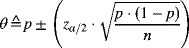$\theta \stackrel{\wedge}{=}p\pm \left(z_{\alpha /2}·\sqrt{\frac{p·(1-p)}{n}}\right)$	confidence interval in the normal approximation to the binomial distribution. (see Equation {6.11})
$\lambda \stackrel{\wedge}{=}{\left(\sqrt{a}\pm \left(z_{\alpha /2}·\frac{1}{2}\right)\right)}^2$	confidence interval in the normal approximation to the Poisson distribution. (see Equation {6.13})
$z=\frac{p-0.5}{\sqrt{\frac{0.5·(1-0.5)}{n}}}$	hypothesis test in a preference study. (see Equation {6.15})

Examples

Suppose we are interested in the occurrence of retinopathy among persons with diabetes. To study this, we randomly select 20 persons from an endocrinology practice who have had adult-onset diabetes for 10 years. Then, we perform an eye examination on these 20 persons. Two of the persons have diabetic retinopathy at this initial examination.1 The remaining 18 persons are examined for retinopathy annually for 10 years. Table 6.1 shows the results of those examinations:

6.1. For which patients did we observe prevalent cases of retinopathy?

Patients LE and AL had prevalent cases of retinopathy. We don't know when they developed retinopathy, only that they had retinopathy at the initial examination.

6.2. For which patients did we observe incident cases of retinopathy?

We consider patients AR, NG, ST, AT, CS, IS, RE, LY, FU, NF, EV, ER, and YO to have had incident cases of retinopathy. We know that they developed retinopathy in the period between examinations.

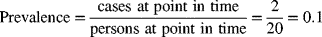
6.3. In the entire sample of 20 persons what was the prevalence of retinopathy at the initial examination?

At the initial examination, the only cases are the two prevalent cases.

$$\text{Prevalence}=\frac{\text{cases at point in time}}{\text{persons at point in time}}=\frac{2}{20}=0.1$$

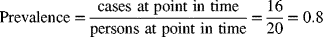
6.4. In the entire sample of 20 persons what was the prevalence of retinopathy at the final examination?

At the final examination, we have the two prevalent cases plus the 14 incident cases.

$$\text{Prevalence}=\frac{\text{cases at point in time}}{\text{persons at point in time}}=\frac{16}{20}=0.8$$

6.5. What is the 10-year risk of developing retinopathy?

For calculating the risk, we only include incident cases in the numerator and exclude the two prevalent cases from the denominator. Those prevalent cases were not “at risk” to be incident cases of disease.

$$\text{Risk}=\frac{\text{new cases over period of time}}{\text{noncases at beginning of period of time}}=\frac{14}{18}=0.78$$

Now, let us think about the incidence of retinopathy. To calculate incidence, we need to calculate the person-time of follow-up. Let us do that for each of the persons in Tables 6.1. For the period during which retinopathy occurred, use the actuarial method to determine person-time.

Table 6.1 Results of 10 annual examinations for retinopathy. Patients with “NE” were not eligible for follow-up, since they had retinopathy at the pre-follow-up examination. “—” indicates a year of follow-up without retinopathy. “X” indicates the presence of retinopathy at the examination at the end of the year.

	Examination
Patient	1	2	3	4	5	6	7	8	9	10
LE	NE
AR	—	—	—	—	—	—	X
NI	—	—	—	—	—	—	—	—	—	—
NG	—	—	—	—	X
ST	—	—	—	—	—	—	—	—	X
AT	—	—	—	X
IS	—	—	—	—	—	—	—	—	—	—
TI	—	—	—	—	—	—	—	—	X
CS	—	—	—	—	—	—	X
IS	X
RE	—	—	—	—	—	X
AL	NE
LY	—	—	—	—	—	—	—	—	—	X
FU	—	—	—	—	—	X
NF	—	—	X
OR	—	—	—	—	—	—	—	—	—	—
EV	—	—	—	—	—	—	X
ER	—	—	—	—	—	—	—	—	X
YO	—	—	—	—	—	—	—	X
NE	—	—	—	—	—	—	—	—	—	—

6.6. Use Table 6.2 to calculate the total person-years of follow-up.

The follow-up times for each subject appear in Table 6.2 . There is no follow-up time for the prevalent cases at the beginning of follow-up. Incident cases were assumed to have occurred, on the average, in the middle of the period before they were recognized as cases. Censored observations (those who never developed the disease) contributed 10 years to the follow-up time. The total follow-up time is 124 person-years.

Table 6.2 Table for calculation of person-time of follow-up.

	Examination
Patient	1	2	3	4	5	6	7	8	9	10	PT
LE	NE										0
AR	—	—	—	—	—	—	X				6.5
NI	—	—	—	—	—	—	—	—	—	—	10.0
NG	—	—	—	—	X						4.5
ST	—	—	—	—	—	—	—	—	X		8.5
AT	—	—	—	X							3.5
IS	—	—	—	—	—	—	—	—	—	—	10.0
TI	—	—	—	—	—	—	—	—	X		8.5
CS	—	—	—	—	—	—	X				6.5
IS	X										0.5
RE	—	—	—	—	—	X					5.5
AL	NE										0
LY	—	—	—	—	—	—	—	—	—	X	9.5
FU	—	—	—	—	—	X					5.5
NF	—	—	X								2.5
OR	—	—	—	—	—	—	—	—	—	—	10.0
EV	—	—	—	—	—	—	X				6.5
ER	—	—	—	—	—	—	—	—	X		8.5
YO	—	—	—	—	—	—	—	X			7.5
NE	—	—	—	—	—	—	—	—	—	—	10.0

6.7. Calculate the incidence of retinopathy.

The incidence is calculated from the number of incident cases and the person-time of follow-up.

$$\text{Incidence}=\frac{\text{new cases over period of time}}{\text{person}-\text{time of follow}-\text{up}}=\frac{14}{124}=0.11\text{cases per person}-\text{year}$$

6.8. To take chance into account for estimates of prevalence, risk, or incidence we usually calculate a confidence interval rather than test a hypothesis. Why is this the case?

A reason we do not usually test hypotheses about prevalence, risk, and incidence is that there is usually no specific value that has biologic relevance. This means there is no sensible null hypothesis to test.

6.9. For the estimate of the 10-year risk of retinopathy, calculate a 95%, two-sided confidence interval using a normal approximation to the binomial distribution.

$$\text{Risk}=p\pm (z_{\alpha /2}ċ\sqrt{\frac{pċ(1-p)}{n}})=0.78\pm (1.96ċ\sqrt{\frac{0.78ċ(1-0.78)}{18}})=0.59\text{to}0.97$$

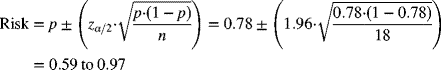
6.10. What is the appropriate interpretation of that confidence interval?

We are 95% confident that the 10-year risk in the population is between 0.59 and 0.97.

6.11. For the estimate of the incidence of retinopathy, calculate a 95%, two-sided confidence interval using a normal approximation to the Poisson distribution.

$$\text{Incidence}=\frac{{\left(\sqrt{a}\pm \left(z_{\alpha /2}ċ\frac{1}{2}\right)\right)}^2}{PT}=\frac{{\left(\sqrt{14}\pm \left(1.96ċ\frac{1}{2}\right)\right)}^2}{124}=0.06\text{to}\mathrm{0}\text{.18 cases per person}-\text{year}$$

6.12. What is the proper interpretation of that confidence interval?

We are 95% confident that the incidence in the population is between 0.06 and 0.18 cases per person-year.

Exercises

6.1. Suppose we are interested in the risk of peripheral neuropathy among persons with diabetes. To study this relationship, we identify 100 persons with a history of diabetes. At an initial examination, three of those 100 persons were found to have peripheral neuropathy. Five years later, the group was reexamined and 12 additional persons were found to have peripheral neuropathy. Based on that information, which of the following is the prevalence of peripheral neuropathy in this group of 100 patients at the end of the five-year study?

1. 0.03
2. 0.07
3. 0.12
4. 0.15
5. 0.17

6.2. Suppose we are interested in the proportion of persons who work for a specific industry who develop chronic obstructive pulmonary disease (COPD). To investigate this relationship, we examine 150 new employees and find that 10 already have COPD. Then, we examine those same 150 persons after they have worked in the industry for 10 years and find 28 new cases of COPD. Which of the following is closest to the point estimate of prevalence of COPD among employees in this industry at the time of the last examination?

1. 0.19
2. 0.20
3. 0.22
4. 0.25
5. 0.31

6.3. Suppose we are interested in the proportion of persons who work for a specific industry who develop chronic obstructive pulmonary disease (COPD). To investigate this relationship, we examine 150 new employees and find that 10 already have COPD. Then, we examine those same 150 persons after they have worked in the industry for 10 years and find 28 new cases of COPD. Which of the following is the 10- year risk of developing COPD among employees in this industry?

1. 0.19
2. 0.20
3. 0.22
4. 0.25
5. 0.31

6.4. Suppose we are interested in the risk of peripheral neuropathy among persons with diabetes. To study this relationship, we identify 100 persons with a history of diabetes. At an initial examination, three of those 100 persons were found to have peripheral neuropathy. Five years later, the group was reexamined and 12 additional persons were found to have peripheral neuropathy. Based on that information, which of the following is closest to the five-year risk of peripheral neuropathy in this group of patients?

1. 0.03
2. 0.07
3. 0.12
4. 0.15
5. 0.17

6.5. Suppose we are interested in the risk of peripheral neuropathy among persons with diabetes. To study this relationship, we identify 100 persons with a history of diabetes. At an initial examination, three of those 100 persons were found to have peripheral neuropathy. Five years later, the group was reexamined and 12 additional persons were found to have peripheral neuropathy. Based on that information, calculate an interval of risk estimates within which we can be 95% confident that the five-year risk of neuropathy in the population occurs. Which of the following is closest to the limits of that interval?

1. 0.02 to 0.22
2. 0.04 to 0.17
3. 0.06 to 0.19
4. 0.08 to 0.17
5. 0.10 to 0.13

6.6. Suppose we are interested in the proportion of persons who work for a specific industry who develop chronic obstructive pulmonary disease (COPD). To investigate this relationship, we examine 150 new employees and find that 10 already have COPD. Then, we examine those same 150 persons after they have worked in the industry for 10 years and find 28 new cases of COPD. Which of the following is closest to the interval estimate for the prevalence of COPD among employees in this industry at the time of the last examination within which we are 95% confident that the population's value is included?

1. 0.18 to 0.32
2. 0.21 to 0.29
3. 0.23 to 0.28
4. 0.24 to 0.26
5. 0.25 to 0.26

6.7. Suppose we are interested in the proportion of persons who work for a specific industry who develop chronic obstructive pulmonary disease (COPD). To investigate this relationship, we examine 150 new employees and find that 10 already have COPD. Then, we examine those same 150 persons after they have worked in the industry for 10 years and find 28 new cases of COPD. Which of the following is closest to the incidence of COPD among employees in this industry?

1. 0.014 per year
2. 0.020 per year
3. 0.022 per year
4. 0.032 per year
5. 0.042 per year

6.8. Suppose we are interested in the risk of peripheral neuropathy among persons with diabetes. To study this relationship, we identify 100 persons with a history of diabetes. At an initial examination, three of those 100 persons were found to have peripheral neuropathy. Five years later, the group was reexamined and 12 additional persons were found to have peripheral neuropathy. Based on that information, which of the following is closest to the incidence of peripheral neuropathy in this group of patients?

1. 0.025 per year
2. 0.026 per year
3. 0.027 per year
4. 0.029 per year
5. 0.032 per year

6.9. Suppose we are interested in the risk of peripheral neuropathy among persons with diabetes. To study this relationship, we identify 100 persons with a history of diabetes. At an initial examination, three of those 100 persons were found to have peripheral neuropathy. Five years later, the group was reexamined and 12 additional persons were found to have peripheral neuropathy. Based on that information, calculate an interval of incidence estimates within which we can be 95% confident that the incidence of neuropathy in the population occurs. Which of the following is closest to the limits of that interval?

1. 0.0 to 0.112 per year
2. 0.001 to 0.056 per year
3. 0.010 to 0.045 per year
4. 0.014 to 0.043 per year
5. 0.008 to 0.048 per year

6.10. Suppose we are interested in the proportion of persons who work for a specific industry who develop chronic obstructive pulmonary disease (COPD). To investigate this relationship, we examine 150 new employees and find that 10 already have COPD. Then, we examine those same 150 persons after they have worked in the industry for 10 years and find 28 new cases of COPD. Which of the following is closest to the interval estimate for the incidence of COPD among employees in this industry within which we are 95% confident that the population's value is included?

1. 0.015 to 0.031 per year
2. 0.017 to 0.039 per year
3. 0.020 to 0.041 per year
4. 0.022 to 0.044 per year
5. 0.025 to 0.030 per year

Note

1. The first examination occurred one year after the initial examination.