Chapter 7
Bivariable Analysis of a Continuous Dependent Variable

7.1 Chapter Summary
7.2 Glossary
7.3 Equations
7.4 Examples
7.5 Exercises

Chapter Summary

In this chapter, we encountered bivariable data sets that contain a continuous dependent variable and an independent variable. In previous chapters, we discussed univariable data sets containing only a dependent variable. In those univariable data sets, our interest was in the dependent variable under all conditions. The independent variable in bivariable data sets, in contrast, specifies special conditions that focus our interest on values of the dependent variable. Continuous independent variables allow us to examine how values of the dependent variable are related to each value of the independent variable along a continuum. Nominal independent variables define two groups of values of the dependent variable between which we can compare estimates of parameters.

The first type of independent variable we examined in this chapter was a continuous independent variable. When we have a continuous dependent variable and a continuous independent variable, we might be interested in estimating dependent variable values that correspond to particular values of the independent variable. When this is our interest, we use linear regression analysis. Alternatively, (or in addition), we might be interested in determining the strength of the association between the variables. With this interest, we use correlation analysis.

Regression analysis can be used to estimate parameters of a straight line that mathematically describe how values of the dependent variable change corresponding to changes in the values of the independent variable. The equation for that straight line includes the intercept (the value of the dependent variable when the independent variable is equal to zero) and the slope (the amount the dependent variable changes for each unit change in the independent variable). The population's intercept is symbolized by α and its estimate from the sample by a. The population's slope is symbolized by β and the sample's estimate by b.

To understand hypothesis testing in regression analysis, it is helpful to understand sources of variation of data represented by the dependent variable. There are three sources of variation, each referred to as a sum of squares or, when divided by its degrees of freedom, as a mean square. The total mean square is the same as the univariable variance of data. The total variation has two components. One component is the variation in values of the dependent variable that is unexplained by the regression line. When this sum of squares is divided by its degrees of freedom, it is called the residual mean square. The other component is the variation in values of the dependent variable that is explained by the regression line. This source of variation is called the regression sum of squares or, when divided by its degrees of freedom (always equal to one for bivariable data sets), it is known as the regression mean square.

The residual mean square is used in estimation of the standard errors used in regression analysis. For hypothesis testing about the population's slope, the standard error is calculated from the residual mean square and the sum of squares of the independent variable.

Hypothesis testing for the slope or intercept uses Student's t distribution. The number of degrees of freedom for that distribution is the number of degrees of freedom used in calculation of the residual mean square (n − 2).

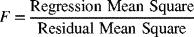
In addition to testing specific hypotheses about the slope and intercept in regression analysis, we can test the omnibus hypothesis. The omnibus hypothesis is a statement that knowing values of the independent variable does nothing to improve estimation of values of the dependent variable. It is tested by examining the ratio of the regression mean square and the residual mean square. This ratio is known as the F-ratio.

The F-ratio has a special distribution known as the F distribution. This distribution is related to Student's t distribution, but it has two, instead of one, parameters for degrees of freedom. One parameter for degrees of freedom is associated with the numerator of the F-ratio (always equal to one when we have one independent variable), and the other is associated with the denominator of that ratio (equal to n − 2 when we have one independent variable). Table B.4 provides values from the F distribution.

When the null hypothesis that knowing values of the independent variable does nothing to improve estimation of values of the dependent variable is true, we expect the F-ratio to be equal to one, on the average. When that null hypothesis is false, the explained variation in values of the dependent variable (i.e., the regression mean square) will be greater than the unexplained variation (i.e., the residual mean square) in those values. Then, the F-ratio will be greater than one. Thus, tests of hypotheses using the F-ratio are all one-tailed.

When we have only one independent variable, the F-ratio also tests the null hypothesis that the slope of the population's regression line is equal to zero. In fact, the square root of the F-ratio, in this case, is equal to Student's t-value that we would obtain if we tested the null hypothesis that the population's slope is equal to zero.

Alternatively, we might be interested in the way values of the dependent variable vary relative to variation in values of the independent variable. A measure of how two continuous variables vary together is the covariance. The covariance is the sum of the products of the differences between each value of a variable and its mean. Covariance has the desirable property of having a positive value when there is a direct relationship between the variables (as values of the independent variable increase, so do values of the dependent variable) and a negative value when there is an inverse relationship between the variables (as values of the independent variable increase, the values of dependent variables decrease). The magnitude of the covariance reflects the strength of the association between the independent and dependent variables.

The covariance, on the other hand, has a distinct disadvantage in that its magnitude is not only a reflection of the strength of the association between the independent and dependent variables, but is also affected by the scale of measurement. This disadvantage can be overcome by dividing the covariance by the square root of the product of the variances of the data represented by the two variables. The resulting value has a range from −1 to +1, with −1 indicating a perfect inverse relationship, +1 indicating a perfect direct relationship, and 0 indicating no relationship between the independent and dependent variables. This value is called the correlation coefficient. We symbolize the population's correlation coefficient with ρ (rho) and the sample's estimate of the correlation coefficient with r.

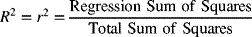
To evaluate the strength of the association between the independent and dependent variables, we square the correlation coefficient. The square of the correlation coefficient (symbolized by R²) is known as the coefficient of determination. The coefficient of determination (or that coefficient times 100%) indicates the proportion (or percentage) of variation in the dependent variable that is associated with the independent variable.

Interval estimation of the correlation coefficient is not very commonly used in health statistics. More often, we encounter tests of the null hypothesis that the population's correlation coefficient is equal to zero (indicating no association between the variables).

Since estimation of the standard error of the correlation coefficient requires estimation of the variances of the data represented by the independent and dependent variables, hypothesis testing involves conversion of the sample's observations to Student's t scale to take into account the influence of chance on those estimates. The number of degrees of freedom for that conversion is equal to the sample's size minus two. Two is subtracted from the sample's size because two variances of data in the population are estimated from the sample's observations.¹

For the correlation coefficient to have relevance, values of both the dependent and independent variables must be randomly sampled from the population of interest. The assumption that the dependent variable is randomly sampled from the population is universal to all statistical procedures. Few procedures assume that the independent variable is also randomly sampled (this is referred to as a naturalistic sample). The value of the correlation coefficient, however, can change dramatically as the distribution of the independent variable in the sample changes (such as can occur when a purposive sample is taken in which the distribution of values of the independent variable in the sample is under the control of the investigator).

A nominal independent variable separates values of the dependent variable into two groups. Comparison of values of the dependent variable between those two groups is accomplished by examining the difference between the means in the groups. The standard error for the difference between means is equal to the square root of the sum of the squares of the standard errors of the means in the groups.

In calculating the standard error for the difference between two means, we often assume that the variance of the data in the two groups is the same. This allows us to use all the observations in our sample to estimate a single variance. That estimate of the variance of data is a weighted average of the separate estimates in each group with their degrees of freedom as the weights. The resulting single estimate of the variance of data represented by the dependent variable is known as the pooled variance estimate.

Under the assumption that the variances of data are equal in the two groups, the pooled estimate of the variance is used in place of individual variances when calculating the standard error for the difference between means.

Hypothesis testing for the difference between means uses Student's t distribution. The number of degrees of freedom is equal to the sum of the degrees of freedom in each of the two groups (n-2).

Glossary

Bivariable Variance – variation in the dependent variable after taking the relationship with the independent variable into account.
Coefficient of Determination – proportion (or percent) of the variation in the dependent variable that is associated with (explained by) variation in the independent variable.
Correlation Coefficient – an index (i.e., adjusted for scale of measurement) of the strength of association between two continuous variables that is equal to −1 for a perfect inverse relationship and +1 for a perfect direct association. A value of 0 means there is no association.
Covariance – a number that reflects the strength of the association between two continuous variables as well as the scales of measurement of the variables. A negative covariance indicates an inverse association, while a positive covariance indicates a direct association.
Direct Association – an association between two continuous variables in which values of the dependent variable increase as the values of the independent variable increase.
F-ratio – ratio of two variance estimates. It is interpreted by comparison with the F distribution.
Homoscedasticity – a state in which the variance of the dependent variable is the same regardless of the value of the independent variable.
Intercept – parameter of a linear relationship that reflects the value of the dependent variable when the independent variable is equal to 0.
Inverse Association – an association between two continuous variables in which values of the dependent variable decrease as the values of the independent variable increase.
Least Squares Estimate – an estimate of a parameter that is selected to minimize the squared differences between observed and estimated values of the dependent variable.
Mean Square – the average variation. Equal to a sum of squares divided by degrees of freedom.
Naturalistic Sample – a sample in which both the dependent variable and independent variable values have been selected at random from the population. See Simple Random Sample
Omnibus Null Hypothesis – the hypothesis that states that the independent variable does not help estimate dependent variable values.
Pooled Estimate – combination of two (or more) estimates to result in a single estimate.
Purposive Sample – a sample in which the researcher determines the distribution of independent variable values. See Stratified Sample
R-squared – the coefficient of determination.
Regression Analysis – estimation of the parameters of a linear relationship between the dependent and independent variables.
Regression Mean Square – the average explained variation in dependent variable values.
Residual Mean Square – the average unexplained variation in dependent variable values.
Restricted Sample – a sample taken from a population in which only persons with specific independent variable values are selected.
Scatter plot – a graphic representation of the relationship between two continuous variables. Values of the dependent variable are listed on the vertical axis while values of the independent variable are listed on the horizontal axis.
Simple Random Sample – a sample taken from a population in which persons are selected without regard to independent variable values. See Naturalistic Sample
Slope – parameter of a linear relationship which reflects how much dependent variable values increase for a one-unit increase in the value of the independent variable.
Stratified Sample – a sample taken from a population in which the probability of being selected from the population differs according to independent variable values. See Purposive Sample.
Strength of Association – consistency with which dependent variable values change in a certain direction and with a certain magnitude as values of the independent variable change.
Sum of Cross-products – the amount dependent variable values differ from their mean times the amount independent variable values differ from their mean. Used in estimation of covariance and the slope.
Sum of Squares – the amount of variation of the dependent variable. Compare to mean square.
Total Degrees of Freedom – the amount of information in a sample that can be used to estimate the univariable variation of the dependent variable. The sample's size minus one.
Total Mean Square – the average variation in the dependent variable without regard to the independent variable. The total sum of squares divided by the total degrees of freedom. The univariable estimate of the variance of the dependent variable. (see Univariable Variance)
Total Sum of Squares – the amount of variation of the dependent variable without taking into account the independent variable.
Univariable Variance – the average variation of the dependent variable without taking the independent variable into account. (see Total Mean Square)
Weighted Average – a method for calculating a pooled estimate. Equal to the sum of each estimate multiplied by a weight that determines the contribution of that estimate divided by the sum of the weights.

Equations

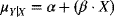$μ_{Y \| X} = α + (β \cdot X)$	linear relationship between the dependent and independent variables in the population. (see Equation {7.1})
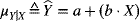$μ_{Y \| X} ≙ \hat{Y} = a + (b \cdot X)$	linear relationship between the dependent and independent variables in the sample. (see Equation {7.2})
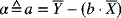$α ≙ a = \bar{Y} - (b \cdot \bar{X})$	estimate of the intercept. (see Equation {7.6})
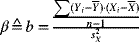$β ≙ b = \frac{\frac{\sum (Y_{i} - \bar{Y}) \cdot (X_{i} - \bar{X})}{n - 1}}{s_{X}^{2}}$	estimate of the slope. (see Equation {7.4})
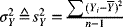$σ_{Y}^{2} ≙ s_{Y}^{2} = \frac{\sum {(Y_{i} - \bar{Y})}^{2}}{n - 1}$	total mean square. Univariable variance estimate. (see Equation {7.9})
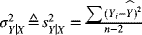$σ_{Y \| X}^{2} ≙ s_{Y \| X}^{2} = \frac{\sum {(Y_{i} - \hat{Y})}^{2}}{n - 2}$	residual mean square. (see Equation {7.10})
$t = \frac{b - β}{s_{b}}$	test of a null hypothesis about the slope. (see Equation {7.11})
$t = \frac{a - α}{s_{a}}$	test of a null hypothesis about the intercept. (see Equation {7.12})
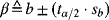$β ≙ b \pm (t_{α / 2} \cdot s_{b})$	interval estimate of the slope. (see Equation {7.13})
$α ≙ a \pm (t_{α / 2} \cdot s_{a})$	interval estimate of the intercept. (see Equation {7.14})
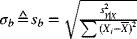$σ_{b} ≙ s_{b} = \sqrt{\frac{s_{Y \| X}^{2}}{\sum {(X_{i} - \bar{X})}^{2}}}$	standard error for the estimate of the slope. (see Equation {7.15})
$F = \frac{Regression Mean Square}{Residual Mean Square}$	F-ratio testing the omnibus null hypothesis. (see Equation {7.17})
$R^{2} = r^{2} = \frac{Regression Sum of Squares}{Total Sum of Squares}$	coefficient of determination. (see Equation {7.20})
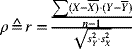$ρ ≙ r = \frac{\frac{\sum (X - \bar{X)} \cdot (Y - \bar{Y})}{n - 1}}{\sqrt{s_{Y}^{2} \cdot s_{X}^{2}}}$	estimate of the correlation coefficient. (see Equation{7.18})
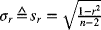$σ_{r} ≙ s_{r} = \sqrt{\frac{1 - r^{2}}{n - 2}}$	standard error of the correlation coefficient. (see Equation {7.21})
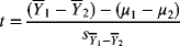
$t = \frac{r - ρ_{0}}{s_{r}}$	hypothesis test for the correlation coefficient. (see Equation {7.22})
$μ_{1} - μ_{2} ≙ {\bar{Y}}_{1} - {\bar{Y}}_{2}$	comparison of two groups of dependent variable values. (see Equation {7.23})
$s_{{\bar{Y}}_{1} - {\bar{Y}}_{2}} = \sqrt{s_{{\bar{Y}}_{1}}^{2} + s_{{\bar{Y}}_{2}}^{2}} = \sqrt{\frac{s_{1}^{2}}{n_{1}} + \frac{s_{2}^{2}}{n_{2}}}$	standard error for the difference between two means not assuming homoscedasticity. (see Equation {7.24})
$s_{{\bar{Y}}_{1} - {\bar{Y}}_{2}} = \sqrt{s_{{\bar{Y}}_{1}}^{2} + s_{{\bar{Y}}_{2}}^{2}} = \sqrt{\frac{s_{Pooled}^{2}}{n_{1}} + \frac{s_{Pooled}^{2}}{n_{2}}}$	standard error for the difference between two means assuming homoscedasticity. (see Equation {7.27})
$σ^{2} ≙ s_{Pooled}^{2} = \frac{\sum (n_{i} - 1) \cdot s_{i}^{2}}{\sum (n_{i} - 1)}$	pooled estimate of the variance as a weighted average of the group-specific estimates with degrees of freedom as the weights. (see Equation {7.26})
$t = \frac{({\bar{Y}}_{1} - {\bar{Y}}_{2}) - (μ_{1} - μ_{2})}{s_{{\bar{Y}}_{1} - {\bar{Y}}_{2}}}$	test of a null hypothesis about two means. (see Equation {7.28})

Examples

Suppose we are interested in the relationship between the basal metabolic rate (BMR) and age in children. To study this relationship, we take a sample of 20 normal children between the ages of 2 and 14 years and measure their BMR. Imagine we observe the results in Table 7.1:

Table 7.1 Basal metabolic rates and age for 20 children

SUBJECT	AGE	BMR
KE	4	52
EP	6	44
ST	8	46
UD	9	47
YI	13	41
NG	7	39
YO	6	41
UR	12	40
EL	10	39
EA	3	56
RN	2	48
IN	8	48
GS	5	44
ST	7	48
AT	2	52
IS	7	44
TI	2	56
CS	4	50
DU	11	39
DE	14	36

7.1 Suppose we want to estimate the mean BMR for children of a specific age. Based on that desire, distinguish between the dependent and independent variables.

We want to estimate BMR so, BMR is represented by the dependent variable. The condition under which we want to estimate BMR is knowing the child's age, making age the independent variable.

7.2 Represent those data graphically as a scatter plot.

We can create a scatter plot in Excel by clicking the Insert tab and selecting a scatter plot. To select your variables, right-click over the graph and choose Select Data. You can label the axes by clicking on the Design tab and clicking on Add Chart Element and selecting Axes Titles.

Figure depicting a scatterplot where the y-axis represents BMR (on a scale of 0–60) and the x-axis represents age (on a scale of 0–15). The data points plotted are represented by black dots. — **Figure 7.1** Scatter plot of BMR as a function of age.

7.3 What equation should we use to describe that relationship mathematically?

The regression equation is:

\hat{Y} = a + (b \cdot X)

Or more specifically:

\hat{B M R} = a + (b \cdot A G E)

7.4 Draw a line on the scatter plot to represent that equation.

To draw a regression line on your scatter plot, right-click on one of the observed values and select Add Trendline. The default will be a straight line.

7.5 Use the scatter plot to estimate the slope of the regression line.

The slope can be estimated most precisely by looking at the most extreme values of the independent variable. These are ages of 2 and 14 years. At two years, the line appears to coincide with a BMR of 52. At 14 years, the line appears to coincide with a BMR of 36. Thus the slope is approximately equal to:

b = \frac{36 - 52}{14 - 2} = - 1.33

7.6 Use the scatter plot to estimate the intercept of the regression line.

The intercept is the BMR for an age of zero (an extrapolation) which appears to be a BMR of about 55.

Next, let us calculate the estimates of the slope and the intercept. To do that, we need to know the sum of squares for both variables and the sum of cross-products. Those are given in the following table:

**Table 7.2** Data from Table 7.1 with calculations for regression analysis

SUBJECT	AGE	BMR	$AGE - \bar{AGE}$	$(AGE - {\bar{AGE})}^{2}$	$BMR - \bar{BMR}$	$(BMR - {\bar{BMR)}}^{2}$	$(AGE - \bar{AGE}) • (BMR - \bar{BMR})$
KE	4	52	−3	9	6.5	42.25	−19.5
EP	6	44	−1	1	−1.5	2.25	1.5
ST	8	46	1	1	0.5	0.25	0.5
UD	9	47	2	4	1.5	2.25	3
YI	13	41	6	36	−4.5	20.25	−27
NG	7	39	0	0	−6.5	42.25	0
YO	6	41	−1	1	−4.5	20.25	4.5
UR	12	40	5	25	−5.5	30.25	−27.5
EL	10	39	3	9	−6.5	42.25	−19.5
EA	3	56	−4	16	10.5	110.25	−42
RN	2	48	−5	25	2.5	6.25	−12.5
IN	8	48	1	1	2.5	6.25	2.5
GS	5	44	−2	4	−1.5	2.25	3
ST	7	48	0	0	2.5	6.25	0
AT	2	52	−5	25	6.5	42.25	−32.5
IS	7	44	0	0	−1.5	2.25	0
TI	2	56	−5	25	10.5	110.25	−52.5
CS	4	50	−3	9	4.5	20.25	−13.5
DU	11	39	4	16	−6.5	42.25	−26
DE	14	36	7	49	−9.5	90.25	−66.5
TOTAL	140	910	0	256	0.0	641.00	−324.0

7.7 Based on those data, what is the sample's estimate of the slope of the regression line?

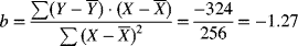
b = \frac{\sum (Y - \bar{Y}) \cdot (X - \bar{X})}{\sum {(X - \bar{X})}^{2}} = \frac{- 324}{256} = - 1.27

7.8 Based on those data, what is the sample's estimate of the intercept of the regression line?

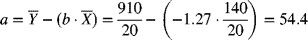
a = \bar{Y} - (b \cdot \bar{X}) = \frac{910}{20} - (- 1.27 \cdot \frac{140}{20}) = 54.4

7.9 How do these values compare with the estimates we made using our scatter plot?

They are very close in value.

7.10 Use the regression equation to estimate the average BMR for 10-year old children in the population.

Y = a + (b \cdot X) = 54.4 + (- 1.27 \cdot 10) = 41.7

7.11 Now use Excel to estimate the slope and the intercept. How do those estimates compare to the ones we calculated by hand?

These computed estimates are the same as the calculated estimates except for rounding.

7.12 Use the Excel output to test the null hypothesis that the intercept is equal to zero in the population (versus the alternative that it is not equal to zero) allowing a 5% chance of making a type I error.

The P-value is much less than 0.05 (4.8x10⁻¹⁷), so we reject the null hypothesis that the intercept is equal to zero and, through the process of elimination, accept the alternative hypothesis that it is not equal to zero.

7.13 Use that output to test the null hypothesis that the slope is equal to zero in the population (versus the alternative that it is not equal to zero) allowing a 5% chance of making a type I error.

The P-value is much less than 0.05 (2.3x10⁻⁵), so we reject the null hypothesis that the slope is equal to zero and, through the process of elimination, accept the alternative hypothesis that it is not equal to zero.

7.14 Use that output to test the omnibus null hypothesis that knowing age does not help to estimate BMR (versus the alternative that it does help) allowing a 5% chance of making a type I error.

The P-value is much less than 0.05 (2.3x10⁻⁵), so we reject the null hypothesis that knowing age does not help estimate BMR and, through the process of elimination, accept the alternative hypothesis that it does help.

7.15 Square the t-value used to test the null hypothesis that the slope is equal to zero. Where in the output can this squared value be found?

The t-value squared is equal to the same value as the F-ratio.

7.16 Another approach to these data would be to estimate the strength of the association between age and BMR. To do that, we can use the R² provided as part of the REG procedure output. What is that value?

The R² in the regression output is 0.6397.

7.17 How can we interpret that R² value?

The R² tells us that 63.97% of the observed variation in BMR is associated with (explained by) variation in ages.

7.18 What do we need to assume before we can interpret that R² as a reflection of the strength of association in the population?

To conclude that 63.97% is an unbiased estimate of the strength of the association in the population, we need to assume that age has been sampled naturalistically (at random) from the population.

Suppose we have a new diet intended to lower serum cholesterol. To investigate this diet, we measure serum cholesterol before and after the diet and record the difference. Table 7.3 shows the changes in serum cholesterol for men and women.

Table 7.3 Changes in serum cholesterol for men and women.

MEN	WOMEN
29	20
36	14
42	20
48	40
37	11
31	45
41	9
31	42
29	22
35	53
48
31
44
32
48
51
22
40
41
43

7.19 Identify the independent and dependent variables.

The dependent variable is the change in cholesterol. That is what we are interested in estimating. The independent variable is gender. That specifies the condition under which we are interested in estimating the change in cholesterol.

Next, we will use Excel to analyze these data assuming homoscedasticity.

7.20 What is the pooled variance estimate?

The pooled variance estimate is listed in the “Equal Variances” output. It is equal to 123.0482143.

7.21 Test the null hypothesis that the difference in serum cholesterol is equal to zero in the population assuming homoscedasticity. As an alternative hypothesis consider the difference in serum cholesterol. Allow a 5% chance of making a type I error.

The appropriate P-value is “P(T<=) two-tail.” That P-value is 0.022816. Since this is less than 0.05, we can reject the null hypothesis that the changes in cholesterol are the same for men and women and accept, through the process of elimination, the alternative hypothesis that the change in cholesterol is different between the genders.

7.22 Test the null hypothesis that the difference in serum cholesterol is equal to zero in the population without assuming homoscedasticity. As an alternative hypothesis assume the difference in serum cholesterol is not equal to zero. Allow a 5% chance of making a type I error.

To answer this question, we have to use the output from the “t-Test: Two-Sample Assuming Unequal Variances” analysis tool.

The appropriate P-value is “P(T<=) two-tail.” That P-value is 0.07748. Since this is greater than 0.05, we fail to reject the null hypothesis that the changes in cholesterol are the same for men and women.

7.23 Which of those two hypothesis tests is more appropriate?

To select the more appropriate result, we can use the “F-Test Two-Sample for Variances” analysis tool.

The P-value is less than 0.05 (0.005034), so we can reject the null hypothesis that the variances are equal and accept, through the process of elimination, that the variances are not equal in the population. This means that appropriate results are from the “t-Test: Two-Sample Assuming Unequal Variances” analysis tool.

Exercises

7.1. Suppose we are interested in the relationship between nerve diameter and nerve conduction velocity. To investigate this relationship, we test 8 nerves of various diameters. These data are in the Excel file EXR7_1.xls on the website accompanying this workbook. Analyze these data as a regression. Based on the results of this analysis, which of the following is the nerve conduction velocity you would expect for a nerve with a diameter of 10 μm?

7.2. Suppose we are interested in the changes in diastolic blood pressure related to age and make the observations in the Excel file called EXR7_2.xls on the website accompanying this workbook. Based on those data, perform a regression analysis. From those results what DBP would we expect, on the average, for persons who are 50 years old?

7.3. Suppose we are interested in the relationship between nerve diameter and nerve conduction velocity. To investigate this relationship, we test 8 nerves of various diameters. These data are in the Excel file EXR7_1.xls on the website accompanying this workbook. Analyze these data as a regression. Based on the results of this analysis, test the null hypothesis that the intercept is equal to zero in the population versus the alternative hypothesis that it is not equal to zero. If you allow a 5% chance of making a type I error, which of the following is the best conclusion to draw?

Reject both the null and alternative hypotheses
Accept both the null and alternative hypotheses
Reject the null hypothesis and accept the alternative hypothesis
Accept the null hypothesis and reject the alternative hypothesis
It is best not to draw a conclusion about the null and alternative hypotheses based on these observations

7.4. Suppose we are interested in the changes in diastolic blood pressure related to age and make the observations in the Excel file EXR7_2.xls on the website accompanying this workbook. Based on those data, perform a regression analysis. Test the null hypothesis that the slope is equal to zero in the population versus the alternative hypothesis that it is not equal to zero. If we allow a 5% chance of making a type I error, which of the following is the best conclusion to draw?

Reject both the null and alternative hypotheses
Accept both the null and alternative hypotheses
Reject the null hypothesis and accept the alternative hypothesis
Accept the null hypothesis and reject the alternative hypothesis
It is best not to draw a conclusion about the null and alternative hypotheses based on these observations

7.5. Suppose we are interested in the relationship between nerve diameter and nerve conduction velocity. To investigate this relationship, we test 8 nerves of various diameters. These data are in the Excel file EXR7_1.xls on the website accompanying this workbook. Analyze these data as a regression. Based on the results of this analysis, test the null hypothesis that knowing nerve diameter does not help estimate nerve conduction velocity versus the alternative hypothesis that it does help. If you allow a 5% chance of making a type I error, which of the following is the best conclusion to draw?

Reject both the null and alternative hypotheses
Accept both the null and alternative hypotheses
Reject the null hypothesis and accept the alternative hypothesis
Accept the null hypothesis and reject the alternative hypothesis
It is best not to draw a conclusion about the null and alternative hypotheses based on these observations

7.6. Suppose we are interested in the changes in diastolic blood pressure related to age and make the observations in the Excel file EXR7_2.xls on the website accompanying this workbook. Based on those data, perform a regression analysis. From the results of the analysis, test the null hypothesis that knowing age does not help estimate diastolic blood pressure versus the alternative hypothesis that it does help. If you allow a 5% chance of making a type I error, which of the following is the best conclusion to draw?

Reject both the null and alternative hypotheses
Accept both the null and alternative hypotheses
Reject the null hypothesis and accept the alternative hypothesis
Accept the null hypothesis and reject the alternative hypothesis
It is best not to draw a conclusion about the null and alternative hypotheses based on these observations

7.7. Suppose we are interested in the relationship between nerve diameter and nerve conduction velocity. To investigate this relationship, we test 8 nerves of various diameters. These data are in the Excel file EXR7_1.xls on the website accompanying this workbook. Analyze these data as a regression. Based on the results of that analysis, which of the following is an interval of values within which we are 95% confident that the slope in the population occurs?

−22.0 to 18.8
−2.9 to 6.9
0.0 to 4.9
2.9 to 6.9
22.0 to 18.8

7.8. Suppose we are interested in the changes in diastolic blood pressure related to age and make the observations in the Excel file EXR7_2.xls on the website accompanying this workbook. Based on those data, perform a regression analysis. From the results of the analysis, which of the following is an interval of values within which we are 95% confident that the slope in the population occurs?

0.42 to 0.57
1.18 to 9.42
2.59 to 21.52
26.35 to 39.2
50.60 to 60.86

7.9. Suppose we are interested in the relationship between nerve diameter and nerve conduction velocity. To investigate this relationship, we test 8 nerves of various diameters. These data are in the Excel file EXR7_1.xls on the website accompanying this workbook. Analyze these data as a regression. Based on the results of that analysis, which of the following is the proportion of variation in nerve conduction velocity that is associated with differences in nerve diameter?

0.756
0.826
0.890
0.923
0.991

7.10. Suppose we are interested in the changes in diastolic blood pressure related to age and make the observations in the Excel file EXR7_2.xls on the website accompanying this workbook. Based on those data, perform a regression analysis. Based on the results of that analysis, which of the following is the proportion of variation in diastolic blood pressure that is associated with differences in age?

0.26
0.44
0.53
0.61
0.78

7.11. Suppose we are interested a diet designed to lower serum cholesterol. When we compare the amount of change in serum cholesterol between men and women we make the observations in the Excel file EXR7_3. Use Excel to test the null hypothesis that the difference of the means of the changes in cholesterol is equal to zero when comparing men and women in the population versus the alternative that it is not equal to zero. If we allow a 5% chance of making a type I error, which of the following is the best conclusion to draw?

Reject both the null and alternative hypotheses
Accept both the null and alternative hypotheses
Reject the null hypothesis and accept the alternative hypothesis
Accept the null hypothesis and reject the alternative hypothesis
It is best not to draw a conclusion about the null and alternative hypotheses based on these observations

7.12. Suppose we are interested in cholesterol levels among patients who had a myocardial infarction (cases) 14 days ago compared to patients who did not have a myocardial infarction (controls). The Excel file containing those data is EXR7_4. Use those data to compare the means between cases and controls. Test the null hypothesis that the difference of the means of the changes in cholesterol is equal to zero when comparing cases and controls in the population versus the alternative that it is not equal to zero. If we allow a 5% chance of making a type I error, which of the following is the best conclusion to draw?

Reject both the null and alternative hypotheses
Accept both the null and alternative hypotheses
Reject the null hypothesis and accept the alternative hypothesis
Accept the null hypothesis and reject the alternative hypothesis
It is best not to draw a conclusion about the null and alternative hypotheses based on these observations

7.13. Suppose we are interested a diet designed to lower serum cholesterol. When we compare the amount of change in serum cholesterol between men and women we make the observations in the Excel file EXR7_3. Use Excel to calculate a 95% confidence interval for the difference between the means. Which of the following is closest to that interval?

−0.10 to 16.13
−0.58 to 15.44
−0.12 to 15.08
0.00 to 15.72
0.92 to 15.26

7.14. Suppose we are interested in cholesterol levels among patients who had a myocardial infarction (cases) 14 days ago compared to patients who did not have a myocardial infarction (controls). The Excel file containing those data is EXR7_4. Which of the following is closest to an interval of estimates of the differences of the mean serum cholesterol between cases and controls within which we can be 95% confident that the population's difference occurs?

−3.2 to 53.5
−1.0 to 44.4
0.0 to 38.2
1.0 to 44.4
3.2 to 53.5