Chapter 2
Measurement: The Alchemist’s Base
Although this may seem a paradox, all exact science is dominated by the idea of approximation. When a man tells you that he knows the exact truth about anything, you are safe in inferring that he is an inexact man. Every careful measurement in science is always given with the probable error … every observer admits that he is likely wrong, and knows about how much wrong he is likely to be.
—Bertrand Russell
In medieval times, scientists mixed, stirred, and poured various ingredients together in their quests to make gold from base metals. Though these alchemists are gone, contemporary men and women have almost as difficult a task as they build concoctions of measurement facts in the search for their truths. Today, measurements and numbers constitute the potion. Just as two people can use the same ingredients yet bake different creations, people can and do use the same measurements to support different conclusions. The illusion we have today is that technology and technique hold the answers. Yet the more we mix, stir, and pour our measurements, the more we may mimic the ancient alchemist’s vain quest. This chapter will begin to show you that in spite of our sophisticated technology, when it comes to measurements, we are not much more advanced than the alchemists.
Measurement is intoxicating. Regardless of where we live, we seem prone to the lure of its charm. Cars, golf carts, boats, and airplanes are equipped with satellite global positioning systems (GPS) showing drivers their movements, speed, and elevation over an onboard map display. Good fishing spots once only known to the seasoned veteran are now accessible to anyone who has a GPS locator. Some golf courses have specially equipped carts with GPS devices that measure the distance, in yards, from the cart to each hole. (The golfers are left on their own to measure the distance from the cart to the ball, unless they have a hand-held GPS device.) If you’re not on a golf course and find yourself lost, don’t worry; your GPS-equipped cell phone will help you navigate the roads and trails of your life, and may well show you the view along the way. While it’s true that in many cases measurement technology has made our world more impersonal, even this is changing. It is now a common service for car manufacturers offer coupled GPS–cellphone-based systems to diagnose car problems remotely, help you find the nearest ATM machine, blink the lights or blow the horn of your car in a large parking lot if you forget where you parked, and automatically signal for help whenever an air bag deploys. All of this is possible because your car’s position and status are being measured.
In many cases, measurements are proudly broadcast. Look around; you’ll find measurements everywhere. Numbers on food packages measure the nutrients and contents, weather forecasting has its color radar pictures, there are gallons per mile statistics on new cars, energy usage statistics on appliances, and just look at all of the energy expended in public opinion polling. There is no doubt that measurement is often regarded as a numerical security blanket. For legal defense, for legal offense, for scientific advancement, for the competitive edge, and just to be nosy, we measure. It’s that simple.
Let’s look first at the one of the most detailed measurements in the world: the measurement of time. On the scale of computer operations, one second is a very, very long time. When it comes to computers, the faster you can divide time, the more instructions you can execute and hence the faster the whole computer works. To find better ways to divide (and measure) time, there is a small group of scientists around the world whose members measure time in incredibly minute fractions of a second.
In the 1950s, “atomic clocks” were invented using cesium atoms where the basic clock was a microwave transition between energy levels [1]. The radiation emitted a microwave of a specific frequency. The accuracy achieved was about 10−10 or 1 second in about 300 years. Not bad—but that was just the beginning. The quest for more accuracy continues today. In 2008, the U.S. National Institute of Standards and Technology unveiled NIST-F1 Cesium Fountain Atomic Clock with an accuracy of about 5 × 10⁻¹⁶, or 1 second in about 60 million years and even higher accuracies measured in experimental prototypes [2].
The interesting part of this work is this question: when you are developing more accurate time measurements, how can you measure something that is potentially more precise than your current standards? The answer: Build two of them and compare their results. Gauging new levels of time accuracy is more than a simple technology challenge. As scientists split time into such small sections, gravitational and special relativity effects become important. And as relativity effects become more important, there may come a time where a complete rethinking of “timekeeping” becomes necessary.
Cybertime machines are a far cry from the first time measurement devices. The height of the sun in the sky, fractions of the moon, and beats of the human heart were among the first ways people measured relatively short times. Today, our everyday measures may not be as precise as cesium fountain clocks but that doesn’t stop us from measuring seemingly everything in sight. Are we better people or, from a societal point of view, are we healthier, happier, more prosperous, and safer because we measure? Think about this question while you are reading this book.
There is no doubt that measurement is essential to understanding and dealing with risk. After all, unless you have “measured” in some way, you would have no understanding or awareness of your surroundings. On the surface, this discussion may sound similar to the old query: “If a tree falls in a forest and no one is around to hear it, does it make a sound?” For a risk-measurement version, we could ask, “If a person is not aware of a risk, does the risk exist?” The answer is yes. Suppose, for example, you were not aware (or in other words had no measure) of the life-saving effects of wearing seat belts. Whether you knew about seat belt safety or not, your risk is still greater than that of a person wearing the belt. In the practical perspective, what you don’t know can hurt you.
But looking at the situation from another point of view, risk management is a rational decision. It requires information. Without measurement feedback to supply the information, there is no risk. This school of thought says that without measurements to supply information about uncertainty, there is no uncertainty, hence no risk. Here, what you don’t know can’t hurt you.
The flaw in this argument is that measurements do not change the actual risk; they only identify it and may give you some indication of its magnitude. What changes with measurement is our perception of the risk. When we “measure” automobile risk, the risk reduction associated with the behavior of wearing seat belts might help us make some of our risk management decisions concerning driving. If we did not know about seat belts, the risk associated with riding in a car wouldn’t be less just because of our lack of knowledge. This is what measurements do for us. In a succinct statement: Measurements alter our perception of uncertainty.
Measurements, perception, and the human mind are inseparable. The seemingly simple process of measurement is a lot more complicated than it seems. We develop one set of measurements based on our initial beliefs; the results alter our perceptions, changing the measurements; and we go around the cycle again. The swamp really gets muddy when the measurements are biased by political agendas, personal prejudices, or the host of other factors that lurk in the dark recesses of our realities.
Not all is bleak, however. There are ways of navigating through the mud to sift out truth from fiction and the biased from the unbiased. There are things to look for: rules for how to differentiate the good from the bad, the precise from the perception of precision, and, of course, fact from fiction.
Measurement has always been and will always be a mix of art and science. Little has changed with the application of technology. Science and computers provide more choices, more types of measurement devices, more data from which to extract information, more capability for precision, more opportunity to succeed, and more opportunity to fail.
Let’s look at a situation that shows exactly how confusing and even deceptive some apparent simple “measurements” can be. When you go to the supermarket to buy poultry and read the “FRESH” label, do you know what this means? Until recently it meant little. But for poultry, it now means the bird was never cooled below its freezing point of 26°F. That’s simple enough, but the industry now has some new terminology that suggests one condition, but means another. For example, “never frozen” legally means the bird was never stored at 0°F or below. Thus store bought turkeys cooled to 1°F are not actually “frozen” according to the U.S. Department of Agriculture [3]. They say that birds stored between 26°F and 0°F may develop ice crystals but won’t freeze all the way through. Unless butchered poultry has some secret internal heating mechanism, I don’t see why birds at stored at 1°F would be “never frozen” yet poultry at 0°F qualify to be labeled “frozen.” This example shows how even simple, yet subtle measurement terms can influence our lives by implying a certain characteristic to the consumer, yet can legally mean a very different thing. Let’s go a little further into the depths of measurement.
MEASUREMENT SCALE
Measuring isn’t always as easy as it sounds. Consider the “gas can paradox.” Suppose you stop at a gas station to fill a 5-gallon gas can. You know it’s a 5-gallon can because its volume is printed on its side. The can was empty when you started. You keep your attention on the pump meter and stop pumping when the pump indicates 5.00 gallons. You look at the can, and it’s not full. You now transfer your attention to the can and stop pumping when the can is full. The pump meter now reads 5.30 gallons. Where’s the error: In the pumping meter or in the size of the can? How could you resolve this problem outside of going to the Bureau of Standards? In essence you can’t. Somewhere in your plan of action, you would have to rely on a standard.
Sometimes standards are not really standards. Here are some examples. If you are putting sugar in your coffee, a teaspoon is a teaspoon. However, if you are administering medication to your 3-year-old, would you be as cavalier in selecting a spoon out of the drawer? Are all so-called teaspoons the same? Check your silverware drawer. If yours is like mine, you’ll find more than one size. And would you be more careful in filling the spoon with your 3-year-old’s medicine than when filling the same spoon with sugar for your coffee?
Now suppose you go to Canada and ask for 5 gallons of gas. Since the Canadian gallon is different than the U.S. gallon, it’s clear that the same names can be used for different standards.
Scale is one of the most important and least appreciated elements of measurement. Sometimes you can’t do anything about it, but at least you should know a little about the concept. A measurement scale implies a standard frame of reference. A measurement without an accepted scale makes conditions ripe for misinterpretations.
There is at least one airline pilot and co-pilot who will always double-check the scale on their fuel load reports before flying. On July 13, 1983, they were flying a Boeing 767 from Ottawa to Edmonton when both engines shut down due to lack of fuel and glided (yes, jets can glide) to a safe landing at an abandoned airport [4]. The number on the fuel load report indicated the flight should have had sufficient fuel for the flight plus a required reserve. As it turned out, the fuel gauges where not functioning for the flight so the ground crew at Ottawa manually checked the fuel quantity with a drip stick. The ground crew then computed the amount of fuel using the standard factor of 1.77 lb/liter that was written on the fuel report form. This was the conversion factor for all other Air Canada aircraft at that time. Here’s the problem: The new (in 1983) Boeing 767 is a metric-based aircraft and the correct conversion factor was 0.8 kg/liter. The flight crew thought they had over 20,000 kg of fuel when in fact they had just over 9,000 kg. At 35,000 ft (10.7 km) with both engines and cockpit navigation instruments shut down, the pilot glided 45 miles (72 km) to safe airport landing. As it turned out, the captain was an accomplished glider pilot, a skill not commonly applied in wide-body jet flying.
I’m sure Air Canada corrected their B-767 fuel forms and in a very short time everyone understood that a different measurement scale needed to be used with this aircraft. Here’s another, and even a more dramatic example of “measurement scale risk” or “measurement scale uncertainty” in the unforgiving world (or universe) of aerospace operations.
On December 11, 1998, NASA launched the Mars Climate Observer [5] from the Kennedy Space Center. The 629 kg (1,387 lb) payload consisted of a 338 kg (745 lb) spacecraft and 291 kg (642 lb) of propulsion fuel. Its mission was to fly to Mars where the main engine would fire for 16 seconds, slowing down just enough to allow the spacecraft to enter an initial elliptical orbit with a periapsis (closest altitude) of 227 km above the surface. Over the next 44 days, “aerobraking” from atmospheric drag on the spacecraft would slow the spacecraft even more and place it in the correct altitude range for its scientific and Mars Lander support missions. That was the plan.
Over the nine months of traveling to Mars the spacecraft’s position and rotation speed was corrected systematically via short impulse thruster burns. Data transmissions from the spacecraft would be fed into trajectory models here on earth and the results would tell the navigation team how to apply the onboard thrusters to make the small midcourse corrections. About a week before Mars orbit insertion, the navigation team determined that the orbit insertion periapsis would be in the 150–170 km range. Shortly before the main engine firing, a recalculation put the initial orbit periapsis at 100 km. While there was serious concern about the trajectory errors, since the lowest survivable altitude was 80 km and little time to determine the cause, the mission was not considered lost. However, 4 minutes and 6 seconds into Mars orbit insertion, the engine was ignited and all communications ended. The communication blackout was expected and it was predicted to last for 21 minutes. The blackout period started 41 seconds earlier than calculated and the spacecraft never responded again. The $324 million mission was lost.
The root cause? Spacecraft navigation information was received at one site and then transmitted to a special team that developed and ran the ground-based trajectory models. They would feed this data into their models and then give the spacecraft navigation team the required vector and thruster impulse information to make the desired course corrections. Just 6 days after the loss of the spacecraft, engineers noticed that the models underestimated the correct values by a factor of 4.45 and this discovery pointed to the problem. One pound of force equals 4.45 Newtons, or 1 lb-sec = 4.45 kg-sec. The spacecraft was designed and operated using the metric scale. The ground-based trajectory models were designed and operated using the English scale. Correcting the final known position, the spacecraft had actually entered an orbit periapsis of 57 km, which was unsurvivable.
Air Canada corrected their latent scale risk and NASA has made considerable program integration changes to ensure something as simple but deadly as data unit inconsistencies will not occur again. Considering the success of the International Space Station, the largest space station ever built, involving equipment, systems, and parts from 16 countries, it appears that measurement scale risk has been effectively managed. Yet with the world converting to metric measures, NASA has decided to stay on the imperial system (pounds and feet) for the next generation of shuttle launch and space vehicles. Their reasoning highlights a common problem in improving legacy systems. The retiring shuttle systems were designed with imperial units and the new shuttle replacement concepts use systems that are derived from the old shuttle. To convert to the metric scale would simply cost too much. So for economic reasons, NASA is going to remain on the imperial scale.
Programs that don’t have these legacy issues will be developed by NASA using metric units. For example, all lunar operations programs will use metric units. So with only the United States, Liberia, and Burma remaining on the imperial measures, the moon will join the majority of earthbound countries in using metric measures. That “one small step for man” and all future steps on the moon will be measured in meters rather than in feet or yards.
Moving to the smaller side of measurement, chaos theory gave the subject a boost toward the esoteric and philosophical when it was first discovered. Chaos scientists realized that, depending on at what level you look at a system, you might see what you believe to be chaos [6]. However, by viewing the same system with a different scale, a definite order can be observed. Thus a seemingly random system really has order and can more easily be understood if we apply a different scale. In plain, down-to-earth English, scale is a generalization and elaboration of the old, well-known concept of seeing the forest or the trees. Or, in the case of chaos theory, seeing jagged lines or the shape of a snowflake—depending on your “scale” of vision.
Think about differences in scale when you look at ocean waves. The number of wavelengths you can observe will vary of course, depending on conditions. On the smallest scale, the wavelengths are less than a foot. On the larger scale, the wavelengths can be measured by movements of the tides.
Scale and measurement are intimately related. You can’t have one without the other. Depending on the measurement scale you use, your results can be totally different. I think you would agree that you can’t predict the weather very well just by looking out of your window; a satellite view gives a better perspective. Every measurement activity has its limitations because it is based upon a given scale. Often this scale can be traced back to a time measure. Just like playing a piece of music on the piano at different tempos, measurement results will change depending on the time scale and frame of reference that is adopted.
Something as simple as the accuracy of the measurement scale shouldn’t be questioned, right? Yet as time changes, our frames of reference sometimes change. Of course, a meter is still a meter. Generally weights and lengths are invariant over time, but some other important scales have changed.
The Scholastic Aptitude Test (SAT), first administered in 1926, has changed its scoring methods. The Educational Testing Service (ETS), the test producer, used an interesting word to characterize the change in scoring. In 1995 they “recentered” both the math and verbal scores, citing facts such as that the abilities of the “average American” are poorer than they were in 1941 and scores have been steadily declining every year. In case you’re wondering why 1941 was selected, it’s because this was the last year the scores were “recentered.” Somehow I don’t think lowering the scale encourages test scores to go up! The lowering of the scores effectively awards the poorer performing students at the expense of the superior students. Thus a combined score (verbal + math) of 1200 in 1994 isn’t quite the same as it is today [7]. The effects of the scale changes are complex and one can understand the technical justifications from reading the literature; regardless of the causes, however, the scale has changed.
The SATs are only one of several gauntlets traversed by students traveling the road to higher education. Another activity designed to qualify high school students for college are the Advanced Placement exams. These courses are taught like regular high school courses for a semester and a standardized test is given at the end of the course. The grading system is 1–5, where 1 and 2 are interpreted as failure and 3 or above may qualify the student to receive college credits. There are a lot of benefits of passing these exams and students have been taking these courses in record numbers. For example, in 2009, 2.9 million students took the exams [8]. This was one record, but there was a second record also set this year. Nationally, more than two out of every five students who took the exams (41.5%) failed, the highest fraction ever. To give you an idea of how many previously have scored poorly, in 2000, 35.7% failed and in 2005, 37.9% failed [9]. Forming a linear trend line from these numbers forecasts the 2009 failure percentage at 39.7%. The message here is the exam failure is increasing faster than at a linear pace. This is some background information for some recent developments in Advanced Placement exam grading.
In the past, students were penalized for guessing. The final score was computed as the number of correct answers minus a percentage of the number of incorrect answers. But starting in the May 2011 exams, scores will only include the number of correct answers [10]. In other words, the penalty for wrong answers (guessing) will be eliminated. This is how the Scholastic Aptitude Test (SAT) is already graded so this change does make the testing guidelines consistent. However, now that guessing has no penalty, the scores can’t be any lower and in fact the total scores should go up. The net effect may not be any different since the 1–5 grading system can still fail the lower 40% of scores but regardless, the scale has changed. The College Board management stated that this change is one part of a major overhaul of their testing instruments and more improvements can be expected in the future.
Two scales that everyone has in common are time and money. Thanks to the magic of our financial markets and a host of other factors, the scale of monetary value is a function of time. By far the best example of changing scale occurred in the early part of 1997 and relates to how the government measures the changing worth of money.
A study unveiled at the end of 1996 from the now infamous Boskin Commission [11] (formally called the Advisory Commission to Study the Consumer Price Index), showed that the Consumer Price Index (CPI), one of the U.S. government’s most important inflationary scales, overstated the cost of living by 1.1 percentage points. This finding was estimated to save about $133.8 billion dollars over the next five years. Since about 30% of the federal budget, including many entitlement programs, is indexed to the CPI, the Wall Street Journal believes the federal government would spend a trillion dollars less than expected over the next decade. You and I save money by tightening our belts and spending less. The federal government saves a trillion dollars by changing a formula. The actual effects of recomputing the CPI evaluated about ten years later suggested [12] that the changes should have been 1.2 to 1.3% in 1996. In 2009, the error was closer to 0.8% but since the CPI is a result of a complex statistical formula involving “stratified random sampling,” there is an inherent uncertainty in any CPI evaluation that doesn’t seem to be mentioned when CPI results are released [13]. Social Security, veteran benefits, and a myriad of other governmental programs are related to this index. The point? Just because a governmental agency has computed a new index value does not mean that it is an exact value. The correct strategy would be to release a range rather than a single number. When you hear and read about changes in economic indicators, think about the possible error or uncertainty in the results. In many cases, with a little scholarship you can also identify the ranges and decide for yourself what the changes really are—if they exist at all.
Measurement standards are not always esoteric subjects. They permeate almost every aspect of life in our global society. Consider the United States’ “national pastime,” major league baseball; more specifically, the size, weight, composition, and performance characteristics of a baseball itself.
The Rawlings Sporting Goods Co. is the official maker of baseballs for both major and minor leagues in the United States. Quality and uniformity are paramount. You may not think that baseball quality control is important, yet to a sport that captures the hearts of millions of people and produces billions of dollars in revenue, the business of baseball is more than a game. Just look at the home run hitting and base hit legacies of baseball’s greatest players. If baseballs weren’t held to tight manufacturing standards, these records would be meaningless.
To ensure that baseball measurements stay the same, Rawlings samples balls from each new production lot made at their plant in Costa Rica. In a room where the environment is maintained at 70°F and 50% humidity, each ball is fired at a speed of 58 mph at a wall of ash wood. This is the same wood as used for making Major League bats. The ball’s speed on the rebound is measured and divided by the initial speed to compute ball’s “coefficient of restitution” (COR). Major League rules state that the balls must rebound at 54.6% of their initial speed, plus or minus 3.2 percentage points. Any faster and the ball has too much spring, any less and the ball has too little.
According to Robert Adair, currently Professor Emeritus at the Yale University Department of Physics and the “official physicist” to the National League in the late 1980s, a batter connects with a home run power hit from a pitcher’s fast ball of 90+ mph in about 1/1000th of a second. The collision between the ball and bat compresses the hard ball to about half of its original size.
In order to routinely manufacture these items, Rawlings uses techniques that are not widely advertised. Yet we know the basics. Each baseball requires about a quarter mile of wool and cotton thread tightly wound around a rubber-covered cork center. If the ball is wound too tightly, it has more bounce, but then exceeds its weight requirements since more material was used in the ball. This example illustrates some of the inherent checks and balances in the measurement process. The end result? Because measurement standards exist, the eligibility requirements to join baseball’s record-breaking elite have changed little over the decades.
In recent years, the influence of performance-enhancing drugs has tainted some baseball record achievers. When questioned about the steroid influence on performance, Professor Adair doubted that the drugs have had a major effect. He stated that historically, weight lifting was not encouraged since the general (incorrect) belief was that the increase in muscle mass would slow reaction speeds. Today, weight training is common and baseball players are generally stronger and bigger than they were in the past. According to Professor Adair, 30 years ago the average baseball player’s weight was about 170 lb. Today the average weight is over 200 lb [14]. So, at least for baseball performance, the measurement scale has not changed due to any changes in the implements of the game. The players have changed.
When performance records are broken, any hint of impropriety can taint the achievements regardless of the veracity of the claims. One thing is certain in baseball: the hitting records are not due to changes in the ball’s performance measurements.
PRACTICAL LAWS OF MEASUREMENT
Aside from scale considerations there are a series of principles you can rely on to help you through the murky waters of measurement. I call them “laws” because as far as I am concerned they’re true, even though no one has ever tried to prove them. Together they’ll give you a tool kit to tackle measurement facts. Use them as a frame of reference and scale to help you decide for yourself how to interpret “the facts.” We’ll discuss them one by one, with some examples that show how the laws work.
Law #1: Anything Can Be Measured
Did you know [15]…
Almost 50% more people fold their toilet paper than crumple it.
68% of Americans lick envelope flaps from left to right (the other 32% do it from right to left).
37% prefer to hear the good news before the bad news
28% squeeze the toothpaste from the bottom of the tube
38% sing in the shower or bath
17% of adult Americans are afraid of the dark
35% believe in reincarnation
17% can whistle by inserting fingers in their mouth
and finally:
20% crack their knuckles
Do you care? You can rely on the fact that somebody does. Just search the Internet for any subject and add the word “statistics” and you can see the diversity of measurements people develop and analyze. This is how new products are created. Market research is a highly competitive, multibillion-dollar industry that measures consumer preferences. We are exposed to its products continuously. For example, let’s examine the fairly mundane subject of soap. What makes you buy one brand instead of another? Its scent? The amount of lather? Its shape? Color? Size? The design on the box? All of these characteristics are a function of consumer preferences that soap manufacturers measure on a continual basis.
Consumer preferences are but a small part of the measurement challenge. As we discuss risk management, you’ll see how much of this subject is dependent on our collective judgments, opinions, and beliefs. The challenge we face is how to use the analytical and technical tools we’ve developed to measure intangible, transient variables such as public risk perceptions.
Technology, coupled with the powers of human creativity, mathematics, statistics, and science, provides the potential to measure virtually anything and everything. Even the most seemingly subjective processes can be measured once the desired results are clearly defined. This means that real measurement decisions are now much more difficult than in the past, and brings us immediately to our second law.
Law #2: Just Because You Can Measure Something Doesn’t Mean You Should
When my son was young, he was delighted every time he got to use my measuring tape. He accepted the tool without question and proceeded to measure everything in sight. Of course, as a 4-year-old, he also used the measuring device for some rather creative purposes for which it wasn’t designed. He had neither an application, nor understanding of any of his “measurements,” but the device was fun to use. This may remind you of certain adults when they are given new toys …
Science, on the other hand, has applications and understanding as solid foundations for measuring value. Every year the best of these works get awards. The most well-known and probably most prestigious of these are the Nobel awards. Noble laureates are the select few whose work has made the most significant advances in applications of our current tools toward the understanding of our universe and the advancement of high ideals. In a way, the Nobel Prize awards represent the ultimate assessment of measurement of an individual or team’s scientific or general work performance.
Yet in early October every year, just before the Nobel Prizes are announced, there is another set of awards also given to researchers whose work represents similar ideals, albeit on the opposite side of the spectrum. These are the Ig Nobel Prizes. In 1991 the U.S.-based organization Improbable Research began awarding research or achievements that “makes people laugh, then think.” The organization has grown in size and international popularity since then and its publications range from a journal-level periodical to web blogs. The Ig Nobel awards are given out by real Nobel Laureates, and represent scientific or otherwise works that “cannot or should not be reproduced.” As you might expect, this “award,” intended for the most part as a good-natured spoof, is not always well received. Here is the list of the 2009 “winners.”
Biology: Fumiaki Taguchi, Song Guofu, and Zhang Guanglei of Kitasato University Graduate School of Medical Sciences in Sagamihara, Japan, for demonstrating that kitchen refuse can be reduced more than 90% in mass by using bacteria extracted from the feces of giant pandas [16].
Chemistry: Javier Morales, Miguel Apátiga, and Victor M. Castaño of Universidad Nacional Autónoma de México, for creating diamonds from liquid—specifically from tequila [17].
Economics: The directors, executives, and auditors of four Icelandic banks—Kaupthing Bank, Landsbanki, Glitnir Bank, and Central Bank of Iceland—for demonstrating that tiny banks can be rapidly transformed into huge banks, and vice versa—and for demonstrating that similar things can be done to an entire national economy.
Literature: Ireland’s police service (An Garda Siochana), for writing and presenting more than fifty traffic tickets to the most frequent driving offender in the country—Prawo Jazdy—whose name in Polish means “Driving License.”
Mathematics: Gideon Gono, governor of Zimbabwe’s Reserve Bank, for giving people a simple, everyday way to cope with a wide range of numbers—from very small to very big—by having his bank print bank notes with denominations ranging from one cent ($.01) to one hundred trillion dollars ($100,000,000,000,000) [18].
Medicine: Donald L. Unger, of Thousand Oaks, California, for investigating a possible cause of arthritis of the fingers, by diligently cracking the knuckles of his left hand—but never cracking the knuckles of his right hand—every day for more than sixty (60) years. He never developed arthritis and therefore concluded that cracking knuckles does not cause arthritis [19].
Peace: Stephan Bolliger, Steffen Ross, Lars Oesterhelweg, Michael Thali, and Beat Kneubuehl of the University of Bern, Switzerland, for determining—by experiment—whether it is better to be smashed over the head with a full bottle of beer or with an empty beer bottle [20].
Physics: Katherine K. Whitcome of the University of Cincinnati, Daniel E. Lieberman of Harvard University, and Liza J. Shapiro of the University of Texas, for analytically determining why pregnant women don’t tip over [21].
Public Health: Elena N. Bodnar, Raphael C. Lee, and Sandra Marijan of Chicago, Illinois, for inventing a brassiere that, in an emergency, can be quickly converted into a pair of protective face masks, one for the brassiere wearer and one to be given to some needy bystander [22].
Veterinary Medicine: Catherine Douglas and Peter Rowlinson of Newcastle University, Newcastle-Upon-Tyne, U.K., for showing that cows that have names give more milk than cows that are nameless [23].
As you can see there is an air of satire in the awards but there also is a very serious aspect of recognizing science and achievements that are on the edge of apparent technical or practical relevance. As eloquently stated in a recent article about the awards, “nature herself doesn’t understand the meaning of trivial” [24].
Trivial or not, in the next law, we recognize that everyone (and every measurement) has their limitations.
Law #3: Every Measurement Process Contains Error
It is important to remember that the act of obtaining a measurement is a process in itself. Even though measurements may be accurate, the overall results of the measurement process may be wrong. There are always some errors involved in the measurement process. Success in measuring requires an understanding of the errors and the magnitude of each. Occasionally, error values turn out to be larger than the value of the measurement. This does not necessarily mean the results are useless. It does strongly suggest, however, the value is a “ball park” result, and not a statement of precision.
There is one line of work in which there is plenty of error, we all have an interest in accuracy, and being “in the ball park” isn’t good enough. NASA’s Near Earth Orbit (NEO) Program identifies and tracks comets and asteroids that pass relatively close to earth. The program’s interests are scientific since these celestial objects are undisturbed remnants of the creation of the solar system about 4.6 billion ago. But NEO, in cooperation with the global astronomical community, also serves as an early warning service for Earth residents for objects that may be on a collision course. Most of the objects that enter our atmosphere have been small rocks providing no more than a streak of light across the sky. However, there are indications that other, larger rocks, a few kilometers wide, have had a significant influence on our world ecosystem and any collision with objects of this size today would change everyone’s day.
Most of the time, we have plenty of warning of impending doom since objects large enough to produce Armageddon can be seen and tracked for years before they would be a problem. While all of us work, sleep, and play, there are people and computers searching the skies looking for new threats and tracking old ones.
On the morning of October 6, 2008, at 6:39 GMT, Richard Kowalski, at the Catalina Sky Survey, discovered a small near-Earth asteroid using the Mt. Lemmon 1.5 meter aperture telescope near Tucson, Arizona [25]. Kowalski reported the finding to the Minor Planet Center (MPC) in Cambridge, Massachusetts, the NASA-funded center that has the responsibility for naming new celestial objects and for the efficient collection, computation, checking, and dissemination of astrometric observations and orbits for minor planets and comets. The object was named 2008 TC3, the information was sent around the world to other astronomers, and the data collection activities began. In total, some 570 astrometric (positional) measurements were made by 26 observatories around the world, both professional and amateur. When scientists at NASA’s Jet Propulsion Laboratory in Pasadena, California, compiled all of the telemetry information from the reporting sites, they realized that they had too much data [26]. Data collected from different telescopes requires that the time clocks on each instrument precisely agree in order to compute 2008 TC3’s position at any instant. The differences in clock synchronization translate into errors in 2008 TC3’s location. And for an object traveling at 17,000 mph, a small error in time means a big difference in position. The initial calculations showed that 2008 TC3 was going to hit Earth, but the big questions were exactly where and when. To reduce the time synchronization errors scientists did not use all of the collected data but selected only a dozen data points from each observatory. This method ensured that no one observatory’s data and consequently no one observatory’s error would dominate the results. The final calculations showed that 2008 TC3 was going to going to impact in the northern Sudan around 02:46 UT on October 7, 2008, just a little over 20 hours after being discovered. The differences between the actual and predicted times and locations are shown in Table 2.1. The quality of these calculations shows that proper management of errors can actually enhance the statistical results.
Table 2.1 2008 TC3 Entry Time and Location Model Comparison with Actual Data
| Event | Atmospheric entry | Airburst detonation |
| Observed Event Time (UT) | 02:45:40 | 02:45:45 |
| Predicted Event Time (UT) | 02:45:38.45 | 02:45:45.13 |
| Observed Long./Lat. (deg.) | 31.4E 20.9N | 32.2E 20.8N |
| Predicted Long./Lat. (deg.) | 31.412E 20.933N | 32.140E 20.793N |
Yet not all data and errors can be so elegantly managed. Here’s an example that will influence how much money you will have in your back pocket or your pocketbook. In 1998, the Congressional Budget Office (CBO) predicted a $1.6 trillion in budget surplus over the next 11 years. They are the first to admit the prediction was made with many assumptions about what the future holds. The biggest problem that would invalidate the surplus estimate was the number and severity of economic recessions during the next 10 years. At the time the CBO made this prediction, they had no recessions in their 10-year forecast. This is where the magnitude of the error becomes very personal, at least to your finances. Economic experts claim that even a mild recession in one year could increase the deficit by $100 billion in a single year. A forecasting error of just 0.1 percentage point slower growth each year over the next 10 years would trim a cool $184 billion off the CBO projected surpluses.
Now fast-forward 10 years. The United States experienced a mild recession in 2001–2002 and shared a global recession starting in 2007 or 2008 (depending on which economist you believe), federal spending has accelerated to record amounts, and budget deficits are at record levels. These assumptions were not in the 1998 forecast.
Yet putting aside our economic theory differences, there is one thing we all can believe in: the uncertainty (or error) of any government forecast. Figure 2.1 displays an excellent representation of what we know implicitly, but the U.S. Congressional Budget Office statisticians presented the “data” in a very precise graph of measurement uncertainty. Even though the graph was published in January 2004, the basic lessons are the same today. The y-axis is the U.S. budget deficit (–) or surplus (+) in trillions of dollars. The multishaded fan represents the range of possibilities. The baseline budget projections—the projections with the highest probabilities—fall in the middle of the fan. But nearby projections in the darkest part of the fan have nearly the same probability of occurring as do the baseline projections. Moreover, projections that are quite different from the baseline also have a significant probability of occurrence. On the basis of the historical record, any budget deficit or surplus for a particular year, in the absence of new legislation, could be expected to fall within the fan about 90% of the time and outside the fan about 10% of the time.
Figure 2.1 Uncertainty of the Congressional Budget Office’s 2004 projections of the budget deficit or surplus under current policies.
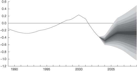
The lesson here is simple. Regardless of whether governmental projections are good or bad news, they are made under a set of assumptions about the future. If government economists could predict the future accurately, chances are they wouldn’t be working for Uncle Sam or anyone else. Since even a small change can alter the numbers drastically, surplus results are only an outcome of a specific scenario and no one knows for sure if the measurement assumptions will turn out to be true. Another interesting property of Figure 2.1 is that the historical results are exact. We know exactly what happened, and consequently there is no uncertainty (or risk) in the past. As Figure 2.1 so eloquently displays, the only uncertainty (or risk) is in the future.
Judge for yourself the likelihood of the government’s track record for economic forecast accuracy and you’ll have an estimate of the likelihood of actually seeing this money. My opinion? This is one case where the size of the error makes politically meaningful surplus or deficit forecasts practically meaningless. And by the way, how many times have you read the final accuracy of budget forecasts after the time period has occurred?
Law #4: Every Measurement Carries the Potential to Change the System
Taking a measurement in a system without altering the system is like getting something for nothing—it just plain doesn’t happen. In particle physics, this law is called the Heisenberg Uncertainty Principle [27]. In 1927, Dr. Werner Heisenberg figured out that if you try to measure the position of an electron exactly, the interaction disturbs the electron so much that you cannot measure anything about its momentum. Conversely, if you exactly measure an electron’s momentum, then you cannot measure its position. Clearly, measurement affects the process here. Even when dealing with the fundamental building blocks of matter, measurement changes the system.
Here’s a more common example. Consider the pressure valve in a bicycle tire. In order to move the needle to calibrate the distance corresponding to the internal tire pressure, kinetic energy must be released. This, in turn, reduces the pressure to be measured. Although the needle mechanism reduces the pressure a negligible amount, it is reduced nevertheless.
As you might expect, electrons and tires are not the only places where this law applies. It’s virtually impossible to have any measuring process not affect what’s being measured.
Here’s another scenario. Nuclear power plants rely on large diesel-powered generators to supply emergency electrical power for reactor operation. The Nuclear Regulatory Commission requires that these generators be started once a month to ensure that they are in good working condition [28]. In reality, the testing itself degrades the useful life of many components. It is likely that testing at this high frequency actually causes the diesel engines to become more unreliable. Some people say that the diesels should be started and kept running. The controversy in this area goes on, but the paradox is real—excessive testing to give the user confidence that the equipment is reliable can actually make the equipment less reliable.
In daily life, this law also recognizes how people react to measurement. Consider the difference in telephone transaction styles between the systems and operators who provide telephone directory assistance and those who answer your calls to exclusive catalogue order services. It’s easy to tell which of the two groups is measured on the number of calls they handle in a day. Each group is providing high-quality service by delivering exactly what the customer expects, yet behaviors differ based on the measurements selected to achieve the desired business results. Imagine the changes that would occur if the performance of Neiman Marcus operators was measured solely by the number of calls each handled per hour. Also, I have observed that in transacting other business over the telephone, when there is a recording saying, “Your call may be monitored for quality purposes,” the people seem more pleasant and helpful. How about you?
Now let’s consider an example of Law #4 from the roads. Some truck drivers are paid by the mile and others are on salary. Tight or impossible schedule promises often force freelance drivers to drive more aggressively. Here speeding, aggressive driving, and long hours at the wheel producing 100,000 miles per year are the behaviors required to survive in the business. Salaried drivers not subject to these tight time schedules produce a radically different driving behavior [29]. You can observe these different behaviors in trucks driving routinely on the interstates. See for yourself.
And nowhere has measurement changed behavior like it has in the world of television journalism. In the early days of TV, newscasting meant a reading of “just the facts” with accompanying on-site footage. The news was a necessary evil as it was often the loss leader for commercial broadcast companies. All of that changed with the success of “60 Minutes.” Suddenly, news became profitable as advertising rates for this show jumped. The measure of news success moved from the mundane but accurate to the entertaining. And that’s where we are. Today, newscasters must worry about ratings as much as other entertainers—sure makes it easier to understand some of the features, doesn’t it?
In recent years, the world of measurement [30, 31] has been introduced to a new discipline, “Legal Citology.” Its founder, Fred R. Shapiro, is an associate law librarian at Yale University. The legal profession uses past cases as building blocks in its work, much as physical scientists use laws and results from previously published experiments in their fields. Inherent in the application and understanding of peoples’ work is the frequency in which people are cited in footnotes. Mr. Shapiro is counting the number of times authors are cited, and he publishes each author’s list [32]. He began doing this in the mid-1980s and the “footnote fever” is running rampant. His count is a pure quantity rather than quality score. However, if you’re a law professor, you’ll want to score high on Shapiro’s Citology scale. Some law schools are using the citation counts in hiring professors. The old academic phrase “publish or perish” has been changed by the Citology score. Now it’s more like “publish something quotable or perish!”
Some people are studying the political aspects of the lists. Professors have noted that the citation counts of white men traditionally failed to acknowledge the work of minorities. Other “researchers” claim that minorities, feminists, and other groups cite each other excessively as a form of “payback.”
Legal Citology measurement has changed the system in a manner I don’t think Fred Shapiro and others ever imagined. One last comment: Shapiro’s citation lists count authors in journals only from 1955 on, because of computer limitations. This is probably just as well, as professors who were working then are now retired. They probably wouldn’t score high anyway. They didn’t have PCs, word processors, email, or the Internet to assist in their quotable writing proliferation.
Law #5: The Human Is An Integral Part of the Measurement Process
There is absolutely no doubt that people influence the measurement process. That is what the Hawthorne Effect [33] and related phenomena are all about. The Hawthorne Effect is the label placed on a study by a Harvard business school professor during the late 1920s and early 1930s. Professor Elton Mayo studied how changes in lighting influenced worker productivity at the Hawthorne plant of Western Electric in Chicago, Illinois. He found that productivity increased not because of lighting changes, but because the workers became convinced of management’s commitment to improve their working conditions and help them be more productive.
Sometimes, however, human interactions with measurements can have just the opposite result of those intended. In early 1994, Tomas J. Philipson, an economist at the University of Chicago and Richard A. Posner, a federal judge in Chicago and a leader in the fields of law and economics, published a book titled: Private Choice and Public Health: The AIDS Epidemic in an Economic Perspective [34]. In the text, the authors argue that widespread testing (measuring) for the AIDS virus may actually contribute to the spread of the disease. They contend “non-altruistic people who have tested positive have no incentive to choose safe sex. On the other hand, those people who have tested negative could use the results to obtain the less cumbersome and easier behavior of unprotected sex.” The authors use an economics analogy, comparing HIV tests to credit checks routinely done on people who want monetary loans. Both are used to increase the likelihood that the person is a good “trading partner.” Just as good credit checks lead to more loan activity, they argue that more HIV testing will lead to more unprotected sexual activity, thereby increasing HIV transmission. Mr. Philipson suggests that “If you didn’t test people, they would be much more careful.”
The authors also take care to state that they have no empirical proof that increased testing leads to, or positively correlates to, the spread of the disease. But they also argue that there isn’t a good statistical case to suggest that widespread testing will reduce transmission either. In essence, the authors’ basic premise regarding human response to testing (measurement) is that sexual activity is a rational activity. You can decide that one for yourself.
Summary Law #6: You Are What You Measure
Sometimes it is impossible to list everything you want to measure in detail. What you really want is to be successful. You have to define the primary measure of that success, and, in business, leave the details to the resiliency and creativity of your employees. Stock, stock options, bonuses, vacations, or a convenient parking spot are some typical motivational tools or “perks” applied to reward and encourage the behaviors required to achieve the desired measurement objectives. This is true for executive compensation as well. If a CEO is being measured on stock price or return on investment, profit, or shareholder equity, then his or her interests and management focus will vary. This is not surprising but it is interesting that from reading corporate annual reports you can often discern from the data which criteria are being used.
The business examples of this law, such as those mentioned in the last paragraph, are fairly straightforward. While there may be subtle details in how the law is applied, the general philosophy is the same. Yet not all applications share this simplicity.
For example, there are two words we use and hear frequently that imply a measurement result. Their use is so common, however, that we seldom question the process that was used, the interpretation of results, or the applicability of the conclusions to our own ways of doing things. These words are “best” and “worst.”
Consider airline on-time performance measurements, published each month by the Department of Transportation to give the public and the airlines feedback on which airlines have and have not been dependable air carriers. Each flight’s departure and arrival times are recorded, sent to a database, compiled by the government, and reported on a regular basis. In the highly competitive environment of airline service, the on-time statistics are powerful (free) marketing material for the “best” and bad news for the “worst.” Yet there is more to this performance measurement than the public sees in the reports. To understand the issues we must go to back in history to the on-time results published for the first quarter of 1996 and shown in Table 2.2.
Table 2.2 Percentage of Flights Arriving within 14 Minutes of Schedule, First Quarter, 1996
Source: U.S. Department of Transportation.
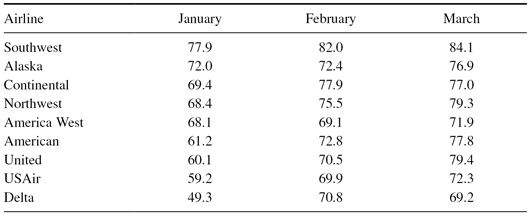
Following the release of these figures, Continental Airlines accused top-ranked Southwest Airlines of fudging its arrival data. These statistics are important because Continental gives bonuses to employees in months where they score in the top three. At Southwest, arrival times are used to determine pilot pay, the connected sequence of subsequent arrival and departure times at airports later in the flying day, and maintenance scheduling intervals. From this point of view, it is clear that major fudging by Southwest could not occur. However, the “on-time derby,” as it has been called, has become so competitive that even small adjustments can change the airline ranking. In the last quarter of 1995, Continental and Southwest were separated by only three-tenths of a percentage point. With this small difference, some people felt that fudging could be done without messing up the airline’s entire schedule. Continental has claimed “numerous inconsistencies” between Southwest’s actual arrival times and the times reported to the Department of Transportation (DOT). This concern was not an isolated instance. It was prevalent throughout the industry for several years [35].
How could Southwest fudge the numbers? Let’s look into how this data was collected. Most major air carriers had equipped their aircraft with an automated system that indicates arrival time by sending an electronic signal to the airline’s computer system when the front door of the plane is opened. By definition, any flight that departs or arrives within 15 minutes of its scheduled time is declared “on time.” The automation takes the human out of the measuring process. So, you might ask, what’s the problem?
Southwest, Alaska, and America West Airlines were the only three major carriers that did not have the automated system. Pilots were responsible for reporting their arrival times—hence the opportunity for changes existed. Human actions were part of the measuring process, competing with automated systems that did not get a penalty or reward for the numbers they reported. Here, both motivation and possibility for error casts doubt on the measurement results. This is especially true when the results between the automated and human-driven systems are very close. Minute differences in watches or clocks could contribute to error even if the planes arrived at exactly the same time. Equipping Southwest’s planes with the automated communications systems of the other airlines would have cost about $5.7 million. To eliminate doubt of Southwest Airline’s performance, management looked at other lower-cost automated solutions they could implement to put them on an even playing field with their very unfriendly competitors.
This is why airline ground and plane crews work hard to get passengers seated and the entrance doors closed. When the door is closed or when the aircraft is moved from the gate, the departure is recorded. The additional time the aircraft may sit on the tarmac before taking off is not used to penalize the “on time” departure data.
Today, technology has leveled the playing field, at least for the data collection aspects of these statistics. Most airlines use what is called the Aircraft Communications Addressing and Reporting System (ACARS) to handle a wide range of functions—including departure and arrival data transmissions. Some utilize a laser guidance system call Docking Guidance System (DGS) that pilots use to park at passenger gates. The manual departure and arrival data transmission is only a backup mode today. The standardization of on-time data has virtually removed the issue that was prevalent in the 1990s among the major airlines.
Now, with the playing field leveled, how could an airline improve its on-time performance? It could maintain a highly reliable aircraft fleet, provide a robust training program to facilitate passenger loading and unloading, and simplify check-in procedures, or it could add a few minutes to its flight time for delays. After all, there is no penalty for being early!
Bill McGee, wrote an insightful article for USA Today in June 2009 [36] stating that unless the distance between seismic plates have shifted dramatically, airlines are now indicating it is taking longer to fly around the country. The CEO of American Airlines, Gerald Arpey, told the shareholders that American was making “strategic adjustments” in an effort to improve customer service. One of the ways American is doing this is to increase its block times.
In this article he reports that, for the route Miami (MIA) to Los Angeles (LAX), the posted block times were: in 1990, 5 hr 45 min; in 1995, 5 hr 25 min; in 2006, 5 hr 30 min and in 2009, 5 hr 40 min. For a shorter flight, from New York (LGA) to Washington, D.C. (DCA): in 1990, 1 hr 15 min; in 1995, 1 hr 00 min; in 2006, 1 hr 16 min; and in 2009, 1 hr 22 min.
It is safe to say that the 2009 aircraft are as fast as, if not faster than, the 1990 versions and that the increase in block time is probably not to due to climate change-induced headwinds. It appears the airlines have done some performance “recentering” of their own that has blurred the line between “best” and “worst.”
It’s easy to state the philosophy of “you are what you measure,” but in situations where there are several attributes being measured, being the “best” in some of them does not necessarily make you the “best” overall. In these very real situations, a decathlon approach may be useful. For example, the “best airline” could be chosen from the summation of airline rankings over several categories, including percentage of on-time departures and arrivals, lost baggage, canceled flights, and customer complaints.
U.S. News and World Report uses the weighted attribute approach when it develops its list of different types of “Top 100” universities. In the ranking process, this publication employs a system of weighted factors that include student retention, faculty resources, student selectivity, financial resources, graduation rate, and alumni giving, along with a number of subfactors. Now if you don’t care about alumni giving or some of the other weighting variables, then U.S. News and World Report rankings are, at best, a guideline in your assessment of school performance. Other published reports tell you the “best” places to live, retire, vacation, and work. They are all compiled from a detailed ranking process that, without an individual’s knowing the details, makes the results useless in practice. The approach, however, is a valid measurement process for situations in which the entity being measured is composed of multiple variables or aspects. After all, you are a complex living organism with a unique personality and a plethora of unique characteristics. How could you expect to measure life’s aspects with a simple tape measure?
Along these lines there is a related phenomenon that seems to be as old as history, where “you are what you measure” takes on genuine results. It is evident in seemingly every area of the human health spectrum, scientifically recognized as real, yet still evades detailed explanation and understanding. I know this introduction sounds ominous, but the process I am about to discuss is a lot more sophisticated and powerful than its simple name suggests. It is the placebo effect.
The word goes back to Hebrew and Chinese origins. Like those of most word etymologies, the string of historical connections of this word is long and diverse. The relatively modern phrase “placebo” has a Latin origin meaning “I shall please” and was used in the Roman Catholic Liturgy. A supplement to Vespers (the evening prayer) was read and prayed when a member of the religious community had died. The text began in Latin with the phrase “Placebo Domino in regione vivorum,” roughly translated as “I shall be pleasing to the Lord in the land of the living” [37].
Medicine has been cutting, poking, bleeding, sweating, and doing other “attention-getting” things to the human body for thousands of years. In many of these seemingly primitive treatment sessions, doctors knew that what they were doing was not directly related to curing the patient. The therapies were placebos. In spite of scientific evidence compiled through the second half of the 19th century, doctors continued to use them because they were pleasing to the patient. The advent of the 20th century saw dramatic improvement in eliminating these torture therapies. Nevertheless, doctors now recognize that placebos play a powerful role in contributing to patient cures. Yet despite almost a century of study, little is known about how placebos actually work.
There is even a great deal of discussion around the definition of a placebo. Here is one that was labeled an acceptable working definition:
A placebo is any therapeutic procedure (or component of any therapeutic procedure) which is given:
(1) deliberately to have an effect, or
(2) unknowingly and has an effect on a symptom, syndrome, disease, or patient but which is objectively without specific activity for the condition being treated.
The placebo is also used as an adequate control in research. The placebo effect is defined as the changes produced by placebos. [38]
The working definition gives you the gist of what a placebo is all about. The general rule of thumb in drug-effect studies is that 20% of the placebo group participants improve from being treated with the “inactive material.” However, there are studies where a remarkable 58% placebo improvement rate has been seen depending on the disease, the placebo used, and the suggestion of the authority [39].
Drug treatments are not the only realm in which the placebo effect is seen. Surgery patients who were enthusiastic about their procedure generally recover faster than do patients who are skeptics. Sure, there are other factors that contribute, but the perception of experience and the psychological factors inherent in dealing with rationally thinking human beings are integral, absolutely inseparable parts of the measurement process.
There are also related health effects for nondrug or -treatment situations. If you’ve been around any workplace recently where people are lifting things, you might see workers wearing support belts designed to reduce the chance of back injuries. In an occupational safety study, researchers found that just wearing the belt made people less prone to injury. This was especially true for the act of lifting, as workers could feel their muscles contracting around the belt area and this feedback would help them use proper techniques. They also found the interabdominal pressure obtained from holding one’s breath had more effect on back support than wearing the belt [40].
Now the net effect is that people who wear the belts have a better chance of not having back injuries, but due to the placebo effect, it is difficult to determine if it is due to the belts or to changes in personal behavior. Since we are talking about psychological measurement, this is a perfect example of how Laws #4 and #5 can be combined. In researching this topic, I came across a simple, precise definition of a placebo [41], one with which I think you will agree: Placebo: A lie that heals.
The placebo effect demonstrates that the human power of perception can be greater than the powers of technology and science put together. Logical explanations of scientific cause and effect can be overwhelmed by the illogical, emotional, and other nonanalytical aspects of the human psyche. We can see the tremendous power of perception and how logical, scientifically acceptable measurement strategies can be ignored due to peoples’ beliefs, values, and internal measurement systems. Summary Law #6 is more than corporate hype or a journalistic sound bite. You, the reader of these words, you are also what you measure.
DISCUSSION QUESTIONS
1. Develop a weighted attribute scoring system to determine the best to worst airline performance from the following data.

Source: U.S. Bureau of Transportation Statistics: January, 2009 through June, 2009.
2. From a newspaper, identify three measurement cases from news stories and discuss the measurement quality and the measurement error.
3. From a newspaper or magazine, identify three measurement cases from the advertisements and discuss the measurement quality and the measurement error.
4. Develop a rating criteria for a “Best Town to Reside” ranking and apply it to 10 towns. Compare your results with those obtained by other groups.
5. Construct three examples for each of the Six Laws of Measurement discussed in the chapter.
Case Study
This case study provides a legal application of laws #4 and #5 (every measurement carries the potential to change the system and the human is an integral part of the measurement process).
Ledbetter v. Goodyear Tire & Rubber Co., Inc., 550 U.S. 618 (2007)
Upon retiring in November of 1998, Lilly Ledbetter filed suit against her former employer, Goodyear Tire & Rubber Co., Inc. (Goodyear), asserting, among other things, a sex discrimination claim under Title VII of the Civil Rights Act of 1964. She alleged that several supervisors had in the past given her poor evaluations because of her gender; that as a result her pay had not increased as much as it would have if she had been evaluated fairly; that those past decisions affected the amount of her pay throughout her employment; and that, by the end of her employment, she was earning significantly less than her male colleagues were. The jury agreed with Ledbetter and awarded her back pay and damages.
The above facts illustrate an example of error or bias in measurements. Upon retirement, Lilly Ledbetter was notified by an anonymous note that her salary was significantly lower than that of her male colleagues with similar experience. This was due to the ripple effect of several biased measurements of her performance throughout her career. She was never aware of such discrimination upon occurrence because of Goodyear’s policy of keeping employee salaries confidential.
On appeal, Goodyear noted that sex discrimination claims under Title VII must be brought within 180 days of the discriminating act. Accordingly, Goodyear contended that the pay discrimination claim was time barred with regard to all pay decisions made before September 26, 1997, or 180 days before Ledbetter submitted a questionnaire to the Equal Employment Opportunity Commission (EEOC). Additionally, Goodyear claimed that no discriminatory act relating to Ledbetter’s pay had occurred after September 26, 1997. The Court of Appeals for the Eleventh Circuit reversed the jury award and held that “because the later affects of past discrimination do not restart the clock for filing EEOC charge, Ledbetter’s claim is untimely.” The U.S. Supreme Court affirmed the Eleventh Circuit, barring Ledbetter from any recovery.
In the context of equal employment opportunities, the laws impose a rigid 180-day limitation on sex discrimination claims. This limitation is essentially a scale for determining the allowable discrimination claims. As a result of this 180-day scale, an employee who was actually discriminated against more than 180 days ago, and did not bring the claim within the 180-day period, was not legally discriminated against. The 180-day limitations period reflects Congress’s strong desire for prompt resolution of employment discrimination matters. The 180-day period appears especially unfair with respect to pay discrimination claims, which naturally take longer to discover.
On January 29, 2009, President Obama signed the Lilly Ledbetter Fair Pay Act of 2009 amending the Civil Rights Act of 1964 to state that the 180-day limitations period starts anew with each discriminatory act.
Case Study Questions
1. From this case study, identify examples or effects of the measurement laws discussed in this chapter.
2. How can employment performance records be checked for measurement bias in practice while maintaining confidentiality?
ENDNOTES
1 Daniel Kleppner, “A Milestone in Time Keeping,” Science, Vol. 319, March 28, 2008, pp. 1768–1769.
2 S. R. Jefferts et al., “NIST Cesium Fountains—Current Status and Future Prospects,” NIST—Time and Frequency Division, Proc. of SPIE Vol. 6673, 667309.
3 USDA Food Safety and Inspection Service Fact Sheet: Food Labeling. September 2006.
4 http://aviation-safety.net/database/record.php?id=19830723-0 (accessed November 8, 2009).
5 Mars Climate Orbiter Mishap Investigation Board Phase I Report, November 1999.
6 Garrnett P. Williams, Chaos Theory Tamed. London: Taylor & Francis, 1997, p. 241.
7 Neil J. Dorans, “The Recentering of SAT® Scales and Its Effects on Score Distributions and Score Interpretations,” College Board Research Report No. 2002–11, ETS RR-02-04.
8 Jack Gillum and Greg Toppo, “Failure Rate for AP Tests Climbing,” USA Today, February 4, 2010.
9 Advanced Placement Report to the Nation 2006, The College Board.
10 Scott Jaschik, “College Board to End Penalty for Guessing on AP Tests,” USA Today, August 10, 2010.
11 “Toward a More Accurate Measure of the Cost of Living: Final Report to the Senate Finance Committee from the Advisory Commission to Study the Consumer Price Index,” December 4, 1996.
12 Robert J. Gordon, “The Boskin Commission Report: A Retrospective One Decade Later,” NBER Working Paper No. 12311, June 2006.
13 Owen J. Shoemaker, “Variance Estimates for Price Changes in the Consumer Price Index”, January–December 2008.
14 Popular Mechanics, March 31, 2008.
15 Mel Poretz and Barry Sinrod, “The First Really Important Survey of American Habits,” Price Stern Sloan, Inc., 1989.
16 Fumiaki Taguchia, Song Guofua, Zhang Guanglei, and Seibutsu-kogaku Kaishi, “Microbial Treatment of Kitchen Refuse with Enzyme-Producing Thermophilic Bacteria from Giant Panda Feces,” Seibutsu-kogaku Kaishi, Vol. 79, No. 12. 2001, pp. 463–469.
17 Javier Morales, Miguel Apatiga, and Victor M. Castano, “Growth of Diamond Films from Tequila,” 2008, Cornell University Library, arXiv:0806.1485.
18 Donald L. Unger, “Does Knuckle Cracking Lead to Arthritis of the Fingers?” Arthritis and Rheumatism, Vol. 41, No. 5, 1998, pp. 949–950.
19 Stephan A. Bolliger, Steffen Ross, Lars Oesterhelweg, Michael J. Thali, and Beat P. Kneubuehl, “Are Full or Empty Beer Bottles Sturdier and Does Their Fracture-Threshold Suffice to Break the Human Skull?” Journal of Forensic and Legal Medicine, Vol. 16, No. 3, April 2009, pp. 138–42.
20 Gideon Gono, Zimbabwe’s Casino Economy—Extraordinary Measures for Extraordinary Challenges. Harare: ZPH Publishers, 2008.
21 Katherine K. Whitcome, Liza J. Shapiro, and Daniel E. Lieberman, “Fetal Load and the Evolution of Lumbar Lordosis in Bipedal Hominins,” Nature, Vol. 450, December 13, 2007, pp. 1075–1078.
22 U.S. patent 7,255,627, granted August 14, 2007.
23 Catherine Bertenshaw [Douglas] and Peter Rowlinson, “Exploring Stock Managers’ Perceptions of the Human-Animal Relationship on Dairy Farms and an Association with Milk Production,” Anthrozoos, Vol. 22, No. 1, March 2009, pp. 59–69.
24 “A Noble Side to the Ig Nobels,” The National, September 26, 2009.
25 http://neo.jpl.nasa.gov/news/2008tc3.html (accessed January 3, 2009).
26 Popular Science, October 2009, pp. 56–57.
27 W. Heisenberg, Über den anschaulichen Inhalt der quantentheoretischen Kinematik und Mechanik. Zeitschrift für Physik, vol. 43, 1927, S. 172–198.
28 “Application and Testing of Safety-Related Diesel Generators in Nuclear Power Plants,” U.S. NRC Regulatory Guide 1.9 Rev 4, March 2004.
29 http://EzineArticles.com/?expert=Aubrey_Allen_Smith.
30 R. B. Jones, Risk-Based Management: A Reliability-Centered Approach. Gulf Publishing, 1995.
31 R. B. Jones, 20% Chance of Rain: A Layman’s Guide to Risk. Bethany, CT: Amity Publishing, 1998
32. Fred R. Shapiro, Collected Papers on Legal Citation Analysis. Fred B. Rothman Publications, 2001.
33 http://www.library.hbs.edu/hc/hawthorne/anewvision.html#e.
34 Tomas Philipson, J. Posner, and A. Richard, Private Choice and Public Health: The AIDS Epidemic in an Economic Perspective, Harvard University Press, 1993.
35 Office of Inspector General Audit Report, U.S. Dept. of Transportation, Report No. FE-1998-103, March 30, 1998.
36 Bill McGee, “Think Flight Times Are Being Padded? They Are,” USA Today, June 29, 2009.
37 Daniel E. Moerman, Meaning, Medicine, and the “Placebo Effect.” New York: Cambridge University Press, 2002, p. 10.
38 Ibid., p. 14.
39 Ibid., p. 11.
40 National Institute for Occupational Safety and Health, “Workplace Use of Back Belts,” NIOSH 94–122.
41 H. Brody, “The Lie That Heals: The Ethics of Giving Placebos,” Annals of Internal Medicine, Vol. 97, Issue 1, July 1982, pp. 112–118.