Chapter 3. Case–Control Studies in Traffic Psychology
Martha Híjar∗, Ricardo Pérez-Núñez∗ and Cristina Inclán-Valadez†
∗National Institute of Public Health, Cuernavaca, Morelos, Mexico
†London School of Economics and Political Science, London, UK
Evidence suggests that for the majority of the world’s population, the burden of road traffic injuries is increasing dramatically. The risk in road traffic derives from the necessity of traveling for different reasons and from a range of factors that determine who uses the different components of the transport system, how and why it is used, and at what times. The concept of risk in road safety includes factors related to exposure, considered as the frequency and time invested in traveling within the transport system by different users or a given population density; the crash probability for a particular exposure; the probability of getting injured after a crash; and the injury as an health outcome. One of the disciplines most often used to identify and measure the weight of each risk factor in traffic injuries is epidemiology. This chapter provides general guidelines on how to use the epidemiological approach to study the problem of road traffic injuries through the case–control study design. It provides a comprehensive description as well as guidelines for when, how, and why this kind of methodological design should be used, in addition to discussing its advantages and disadvantages. We believe that the inclusion of this chapter in this book reflects the need to increase road safety efforts through evidence-based decisions, and that the best way to achieve this is through well-designed research.
1. Introduction
Although the effects of urbanization and industrialization in most countries suggest a degree of inevitability, substantial reductions in rates of road crash fatalities have been achieved in high-income countries despite increasing motorization. Evidence suggests that for the majority of the world’s population, the burden of road traffic injuries is increasing dramatically (Ameratunga, Hijar, & Norton, 2006). Risk in road traffic derives from a need to travel for different reasons and from a range of factors that determine who uses different parts of the transport system, how it is used and why, and at what times (Tingvall, 1997).
The concept of risk in road safety includes factors related to exposure, considered as the amount of movement or travel within the transport system by different users or a given population density; the crash probability given a particular exposure; the probability of being injured after a crash; and the outcome of injury. It has been documented that, although it might not be possible to eliminate all risks, it is possible to reduce the exposure to risk of severe injury or minimize its intensity and fatal consequences.
The global and concerted approach required must consider the wider societal burden of road traffic crashes (both fatal and nonfatal outcomes) and particularly focus on efforts to protect vulnerable road users (e.g., motorcyclists, human-powered vehicles, and pedestrians). Addressing the disparities in both the impact of and response to this problem must be high on the global public health policy and research agenda (Ameratunga et al., 2006).
A substantial body of literature points to the propensity of some road user groups, particularly pedestrians and those using motorized and nonmotorized two-wheelers, to be vastly overrepresented among crash victims at the global level (Peden et al., 2004 and Razzak and Luby, 1998) and be at higher risk of crash-related disability (Mayou & Bryant, 2003). Passengers in formal and informal modes of public and mass transport constitute another important road user group that is a common feature among road crash data, especially from less resourced environments.
Error by a road user may indeed trigger a crash but may not necessarily be its underlying cause. In addition, human behavior is governed not only by individual knowledge and skills but also by the environment in which the behavior takes place (Khayesi, 2003). Indirect influences, such as the design and layout of the road, the nature of the vehicle, and traffic laws and their enforcement or lack of enforcement, affect behavior in important ways. For this reason, the use of information and publicity on their own is generally unsuccessful in reducing road traffic collisions (Allsop, 2002, European Road Safety Action Programme, 2003 and Impacts Monitoring Group in the Congestion Charging Division of Transport for London, 2003). Error is part of the human condition. Aspects of human behavior in the context of road traffic safety can certainly be altered. Nonetheless, errors can also be effectively reduced by changing the immediate environment rather than focusing solely on changing the human condition (Wang et al., 2003).
This chapter provides general guidelines on how to use the epidemiological approach to study the problem of road traffic injuries using the case–control study design. The chapter begins with a general description of epidemiological study designs. It proceeds to give a more comprehensive description of case–control studies, specifically how these studies are defined and when they are most commonly used, followed by “case” definition and alternatives to select cases. Subsequently, it presents the definition of a “control” and explains how controls can be identified and selected. Reasons to match are then presented, followed by a discussion of the forms of matching and stratification and of the disadvantages of matching strategies. An argumentation on how many controls should be included in case–control studies is then presented, followed by a discussion on how to analyze case–control studies and what measures of association–causality are used in this type of study. Several variants of case–control studies are presented. Next, the chapter addresses the problem of representativeness and discusses some of the principal biases that are relevant and characteristic of case–control studies, especially in road safety research and analysis. Finally, the advantages and disadvantages of case–control studies are discussed.
2. Epidemiological Study Designs
The purpose of epidemiology is to describe and explain the population health dynamics—to identify the elements that compose it and to understand the forces that governs it in order to develop actions aimed to preserve and promote health between populations (Hernández-Ávila & López-Moreno, 2007). It is thus not only concerned with the occurrence of disease or other health-related events but also with the identification of factors that cause those conditions, which has become the main focus of modern epidemiology (dos Santos-Silva, 1999b). In general, researchers studying road safety attempt to answer the following questions:
1. Does alcohol consumption increase the risk of pedestrian injuries (Haddon, Valien, McCarroll, & Umberger, 1961)?
 |
2. Does seat belt use decrease the risk of severe road traffic injuries in a car collision (Híjar-Medina, Flores-Aldana, & Lopez-Lopez, 1996)?
 |
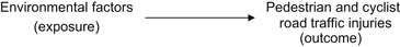
3. What environmental factors could increase the risk of pedestrian and cyclist road traffic injuries (Kraus et al., 1996)?
 |
| Type of study | Assignation of Exposition | No. of Observations (Measurements) by Individual | Selection Criteria of Population under Study | Temporality of Analysis | Unit of Analysis |
|---|---|---|---|---|---|
| Experimental | Controlled (random) | Two or more | None | Prospective | Individual or group |
| Pseudo-experimental | For/by convenience | Two or more | None | Prospective | Individual or group |
| Cohort | Out of the control of researcher | Two or more | Exposition | Prospective or retrospective | Individual |
| Cases and controls | Out of the control of researcher | One or more | Effect | Prospective or retrospective | Individual |
| Crossover | Out of the control of researcher | One | None | Retrospective | Individual |
| Ecological | Out of the control of researcher | Two or more | None | Retrospective | Group or population |
1. Assignation of exposure: observational, experimental, and Quasi-experimental.
2. Number of measurements performed in each study subject to verify changes in the occurrence of both exposition and its effect (longitudinal versus crossover study design).
3. Criteria employed to select population under study (none, exposition, and effect).
4. Temporal relationship between the start of the study and the measurement of the occurrence of the effect (retrospective, prospective, mixed, or ambispective).
5. Unit of analysis for which all variables of interest are measured (individual, group, and population). It is important to note that the concept of an individual in road safety research has not been reduced to a single person. Some studies have also had as a unit of analysis streets (Kraus et al., 1996), street crossing locations (Koepsell et al., 2002), crash sites (Wintemute, Kraus, Teret, & Wright, 1990), etc.
The previous classification categorizes epidemiological studies according to the strength of evidence that each study design provides to the causal relationship between exposure variables and a health outcome of interest (Hernández-Ávila & López-Moreno, 2007). In this sense, the best study design to establish cause-and-effect relationships is the experimental randomized design. For strictly medical interventions, the “gold standard” is the double-blind, randomized controlled trial. This study design involves the random allocation of different interventions (treatments or conditions) of studied subjects to compare treatment groups with control groups not receiving the treatment. Participants, caregivers, or outcome assessors are not allowed to know which intervention are they receiving. Although these studies may be ideal for testing the efficacy of interventions, there are many instances in which trials would be impossible, impractical, and/or unethical. For example, it would generally be considered unethical to randomly assign research subjects to be exposed to alcohol in order to evaluate the substance’s effects on their driving ability.
In this sense, the choice of study design is affected by numerous factors and considerations. According to Robertson (1992), this decision depends on
what is the unit of analysis (people, vehicles, environment)? In what population should the study be conducted? To what population of people, vehicles, or environments will the results be generalized? What kind of measurements of the factors are available or could be obtained? How reliable and valid are the measurements? Can the data be collected without violating ethical guidelines? How can the study isolate the effects of given factors independent of, or in combination with, other relevant factors? How much time will be needed to complete the study? How much will the study cost? (pp. 84–85)
3. Case–Control Studies
3.1. Definition and Characteristics
Case–control studies represent a sampling strategy in which the population under study is selected based on the presence (case) or absence (control) of an event of interest (i.e., health condition, disease, and death) (Lazcano-Ponce, Salazar-Martinez, & Hernandez-Avila, 2001). The underlying purpose of these studies is to identify causal factors of the events of interest by comparing characteristics of both groups (cases and controls). As shown in Figure 3.1, case–control studies start by identifying the study population, from which cases are identified and their exposure status is determined retrospectively. Then, a control group of study subjects is sampled from the entire source population that gives rise to the cases (Rothman & Greenland, 1998). Once the exposure status is also identified in the control group, comparison between both groups may evidence whether exposure to a specific factor is higher in the case group (risk factor) or lower (protective factor) or the same as in the control group (no evidence of association) (dos Santos-Silva, 1999a and Hernández-Ávila and López-Moreno, 2007). It is important to remember that assignation of exposure in case–control studies is out of the control of researchers.
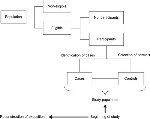 |
| FIGURE 3.1 |
A good example of a case–control study in road safety is the study of Jones, Harvey, and Brewin (2005). This study explored the symptom profiles of acute stress disorder and post-traumatic stress disorder (PTSD) in participants who did or did not sustain traumatic brain injury following a road traffic accident. This study selected as “case” all survivors of a road traffic collision during a period of time who had been diagnosed with traumatic brain injury (TBI). The control group was composed of survivors of a road traffic accident during a period of time with no TBI (Jones et al., 2005). Once the exposure status was identified, comparison between both groups could evidence whether exposition to a specific factor is higher in the case group (risk factor) or lower (protective factor) or the same as in the control group (no evidence of association) (dos Santos-Silva, 1999a and Hernández-Ávila and López-Moreno, 2007). This study found that at 3 months post-trauma, there was no difference in PTSD symptom profile between non-TBI (controls) and TBI groups (cases).
Case–control studies can be conceptualized within the framework of a hypothetical cohort study (Rothman & Greenland, 1998). Although in practice it can be difficult to characterize the cohort or study base (Wacholder, McLaughlin, Silverman, & Mandel, 1992), case–control studies can be based on special cohorts of interest rather than on the general population (Rothman & Greenland, 1998).
3.1.1. When Are Case–Control Studies Used?
Case–control studies are frequently one of the first approaches used in the etiological study of a disease or health condition. This is in part due to the possibility of incorporating in the analysis many exposition factors simultaneously and relatively quickly and inexpensively (dos Santos-Silva, 1999a). Therefore, case–control studies represent a cost-effective way of identifying risk and protective factors and generating hypotheses for subsequent, methodologically stronger studies (Lazcano-Ponce et al., 2001). Case–control design is simply an efficient sampling technique for measuring exposure–disease associations in a cohort or study base (Wacholder, et al., 1992). In addition, case–control studies are commonly used to study conditions that are relatively rare or that have a prolonged induction period (dos Santos-Silva, 1999a).
A study carried out in Shanghai, China, is an example of a case–control study measuring the effect of exposition to different risk factors (Yu, Wang, & Chen, 2005). This study explored the risk factors influencing the occurrence of road traffic injuries on drivers with a history of accidents and on controls. The study included physiological, psychological, and behavioral risk factors and found that factors such as tiredness and waking up early were related to the occurrence of road traffic injuries.
It is important to highlight that the human host or vector (pedestrian and driver) in road traffic injuries has been the unit of analysis in most case–control studies, to the neglect of factors that may be more subject to change for injury control. However, case–control designs can also provide strong evidence regarding environmental factors (Robertson, 1992).
3.2. Case Definition
As can be seen in the previous examples, the definition of a case can be virtually anything that the investigator wishes: an injured person from a specific gender or age group or a specific road user—pedestrian, cyclist, motorcyclist, or car occupant. Whoever the case is, the case definition will implicitly define the source population for cases, from which also the controls should be drawn (Rothman & Greenland, 1998). In this sense, having precise criteria to define a case is highly relevant.
Objective documentation that cases actually have the disease or health condition under study is highly recommended. When this is not possible, an alternative is to classify cases as “confirmed,” “probable,” or “likely.” If analysis shows a gradual decrease in relative risk from the confirmed category to the likely category, problems of erroneous classification are suspected. For this reason, this classification gives researchers the opportunity to evaluate the probability that results are affected by an incorrect classification of the disease analyzed (dos Santos-Silva, 1999a).
In general, there are two types of cases: incident and prevalent. Incident cases are those new cases that appear in the population under study in a specific period of time (or during a pre-established period of time). Memory of past events and exposures tends to be more accurate in cases recently diagnosed. For this reason, incident cases are preferred over prevalent cases. In addition, it is less probable that incident cases changed their habits (exposures) as a result of disease. Prevalent cases are all cases existent (new and previous) in a population in a specific time (or a short period of time) (dos Santos-Silva, 1999a). Prevalent cases are especially useful when it is not possible to establish a specific date for disease onset. However, patients with a condition of prolonged duration tend to be overrepresented because those with a condition of short duration drop out of the study due to recovery or death. Unless exposure under study is not related to recovery or survival, incident cases should be privileged when designing a case–control study (dos Santos-Silva, 1999a).
3.2.1. Identification and Selection of Cases
Selection of cases should privilege internal validity rather than external validity (dos Santos-Silva, 1999a). Internal validity refers to the absence of errors made during the selection process of the population under study or during the measurement of individual variables of interest. To achieve internal validity, comparability of groups under study should be met (Hernandez-Avila, Garrido, & Salazar-Martinez, 2000). On the other hand, external validity refers to the capacity of a study to generalize observed results to the base population. A prerequisite of external validity is the achievement of internal validity. This is the reason why internal validity should be privileged over external validity (Hernandez-Avila et al., 2000).
In addition, selection of cases should include only those for whom the reasonable possibility exists that the disease or health condition existed prior to the study (dos Santos-Silva, 1999a). Ensuring that cases comprise a relatively homogeneous group will increase the possibility of detecting important etiological relations. It is less important to be able to generalize results to the entire population than to establish an etiological–causal relation even when this relation only applies for a small group of the population (dos Santos-Silva, 1999a).
Ideally, selection of cases should follow the paradigm of longitudinal studies. It is recommended to select recently diagnosed cases (incident cases). Less recommended is the use of prevalent cases unless other requisites are met or when justified (Table 3.2; Lazcano-Ponce et al., 2001).
| OR, odds ratio; RR, relative risk. | |
| Option | Characteristics |
|---|---|
| Utilization of incident cases with long exposure periods or prolonged latency periods | OR tends to be similar to RR when cases under study are incident and preceded by a long-term exposure. |
| Use of prevalent cases with prolonged exposure period | OR is similar to RR if disease does not affect the status of exposure and there is a long-standing exposure period. Prevalent cases could be included, especially when new cases are not available (low prevalent conditions), lethality of disease is low, and exposure does not modify the clinical outcome of the disease (survival). |
| Utilization of incident cases and very short exposure periods | OR is similar to RR when the risk period is short and incident cases are used. |
| Utilization of prevalent cases | OR comes closer to RR when prevalence of cases is low only if outcome is not related with survival before selection, condition, or exposure and if disease does not affect the exposure status. |
| Utilization of death cases | Inclusion of death cases is only justified in exposures that could be quantified through the use of high-quality secondary sources of data, such as medical records and occupational information sources. |
Commonly used sources of cases in the published literature on road traffic injuries are hospital cases (Celis et al., 2003 and Tester et al., 2004), administrative registries such as city police reports (Lightstone et al., 1997 and von Kries et al., 1998), and coroners’ registries (Wintemute et al., 1990). Also common is a combination of sources (Stevenson, Jamrozik, & Burton, 1996).
Even when cases are identified exclusively at hospital points, they can be reasonably assumed to represent all cases in a region or determined study population when, for example, the severity of the condition or disease requires hospitalization. This is the case for severe road traffic injuries, for which health care utilization patterns are different from those of most other diseases due to the severity of injuries and because the urgent demand for treatment eliminates some of the most common access barriers (Híjar-Medina & Vázquez-Vela, 2003). However, slight injuries that are treated in a hospital or emergency room cannot be considered as representative of the total study base.
When reporting results of a case–control study, it is important to specify which cases were not included in the study even though they satisfied all inclusion criteria. Reasons for exclusion and the number of cases by reason should be specified. This information allows the assessment of the level to which study results may be affected by a selection bias (dos Santos-Silva, 1999a).
3.3. Definition of a Control
A control is an individual without the condition of interest who serves as reference for a case. The purpose of the control group is to determine the relative (as opposed to absolute) size of the exposed and unexposed denominators within the source population. From the relative size of the denominators, the relative size of the incidence rates (or incidence proportions, depending on the nature of the data) can be estimated (Rothman & Greenland, 1998). Thus, case–control studies yield estimates of relative effect measures (Rothman & Greenland, 1998).
It is important to note that controls should meet all eligibility criteria defined for cases other than those related to the diagnostic of disease, outcome, or health condition under analysis (dos Santos-Silva, 1999a).
3.3.1. Identification and Selection of Controls
Conceptually, it can be assumed that all case–control studies are nested inside a particular population (dos Santos-Silva, 1999a). This is called the “study base,” which can also be thought of as the members of the underlying cohort or source population for the cases during the time periods when they are eligible to become cases (Wacholder, et al., 1992). However, the identification of the appropriate study base from which to select controls is the primary challenge in the design of case–control studies (Wacholder, et al., 1992). For this reason, selecting a control group could be the most difficult part of a case–control study (dos Santos-Silva, 1999a). Controls are selected from the same population base as cases but through a mechanism independent from that used for case selection (Hernández-Ávila & López-Moreno, 2007).
Some authors have set basic principles for control selection that are required to minimize bias, including the following:
• Cases and controls should be “representative of the same population base experience” (Wacholder, et al., 1992, p. 1020). Operationally, this implies that if a control develops the condition or disease (the event under study), he or she must be included as a “case” in the study (Lazcano-Ponce et al., 2001).
• Confounding should not be allowed to distort the estimation of effect. This is referred to as the deconfounding principle. Confounders that are measured can be controlled in the analysis. Unknown or unmeasured confounders should have as little variability as possible. Because this variability is measured conditionally on the levels of other variables being studied, the use of stratification or matching can, in effect, reduce or eliminate the variability of the confounder (Wacholder, et al., 1992).
• Controls must be sampled independently of their exposure status to ensure that they represent the population base (Rothman & Greenland, 1998).
• The degree of accuracy in measuring the exposure of interest for the cases should be equivalent to the degree of accuracy for the controls, unless the effect of the inaccuracy can be controlled in the analysis (Wacholder, et al., 1992).
• The probability of selection of a control should be proportional to the time a subject has remained eligible to develop the event or condition under study. This implies that not only are all controls at risk of developing the condition but also subjects selected as controls in an early stage could become cases in latter stages (Lazcano-Ponce et al., 2001).
• The study should be implemented so as to learn as much as possible about the questions being investigated for a fixed expenditure of time and resources (Wacholder, et al., 1992). This has been called the efficiency principle, and it calls for consideration of costs as well as validity in selection of controls. Statistical efficiency refers to the amount of information obtained per subject; more broadly, efficiency encompasses the time and energy needed to complete the study (Lazcano-Ponce et al., 2001 and Wacholder et al., 1992).
• An exclusion rule that applies equally to cases and controls is valid because it simply refines the scope of the study base (Wacholder, et al., 1992).
3.3.1.1. Source of Controls
Most of the sources of controls for epidemiological research are presented in Table 3.3 along with their advantages and disadvantages. However, studies of road traffic injuries commonly use controls obtained from hospitals and neighborhoods. For example, as discussed previously, one of the most popular and practical strategies to identify road traffic injury cases is through a hospital or emergency room. It could be difficult to consider that they represent all persons injured as a result of road traffic collisions, although this may be true when a hospital covers the entire population under study and there are no access barriers for individuals. If not, they might be claimed to be representative only of road traffic injury users of a specific hospital or emergency room. Controls, however, may sometimes be difficult to identify in the context of this design. For example, what would be a good control for an injured motorcyclist or car occupant? One solution is to select users of the same medical unit who are more comparable to cases with respect to quality of information because they also have been ill and hospitalized (Wacholder, Silverman, McLaughlin, & Mandel, 1992a). They are also the most convenient choice when controls will be asked to provide bodily fluids or to undergo a physical examination (Wacholder, et al., 1992a).
| Type of Controls | Advantages | Disadvantages |
|---|---|---|
| Population controls | Same study base: Ensures that the controls are drawn from the same source population as the case series. Exclusions. Definition of the base can encompass the exclusions. Extrapolation to base population: Distribution of exposures in the controls can be readily extrapolated to the base for purposes such as calculations of absolute or attributable risk. | Inappropriate when there is incomplete case ascertainment or when even approximate random sampling of the study base is impossible because of nonresponse or inadequacies of the sampling frame. Inconvenience: Definition of the base can encompass the exclusions. Recall bias: Responses by a previously hospitalized case may reflect modifications in exposure due to the disease, such as drinking less coffee or alcohol after an ulcer, or due to changes in perception of past habits after becoming ill. Less motivation to cooperate. |
| Random digit dialing | In some circumstances, could come close to sampling randomly from the source population. | Probability of contacting each eligible control will not necessarily be the same because households vary in the number of people who reside in them and the amount of time someone is at home. Contact with a household may require many calls at various times of day and various days of the week. Challenging to distinguish business from residential telephone numbers. |
| Neighborhood controls | Convenient substitute for population-based sampling of controls. Control of environmental or socioeconomic confounding factors. | If a person is injured in a neighborhood, controls who have knowledge of the injury may give misleading information because of denial of personal vulnerability or other psychological factors. Overmatching. Could introduce selection bias because it cannot be assumed that controls represent the base population from which cases were extracted. |
| School rosters | Especially useful when population under study is of school age. | Selection bias in contexts of high rates of school desertion. |
| Hospital or disease registry controls | Comparable quality of information. Convenience. Factors such as socioeconomic characteristics, race, and religion can be controlled. Normally, they tend to be willing to participate and to provide complete and exact information. | Different catchments: Catchments for different diseases within the same hospital may be different. Berkson’s bias: Caused by selection of subjects into a study differentially on factors related to exposure. Disease of controls could be related to exposure (risk factors). |
| Other diseases obtained from a population registry | Comparable quality of information. Willing to participate and to provide complete and exact information. | Berkson’s bias: Caused by selection of subjects into a study differentially on factors related to exposure. Disease of controls could be related to exposure (risk factors). |
| Controls from a medical practice | Useful strategy when it is otherwise difficult to find controls who are comparable to cases on access to medical care or referral to specialized clinics. | The study base principle can be jeopardized with medical practice controls because the exposure distribution for controls may not be the same as that in the study base. |
| Friend controls | More convenient and inexpensive source of controls. Controls can be selected from a list of friends or associates obtained from the case at little extra effort while the case is being interviewed. Friends may be likely to use the medical system in similar ways. Moreover, biases due to social class are reduced because usually the case and friend control will be of a similar socioeconomic background. Despite serious shortcomings, friend controls may be useful in some exceptional circumstances, such as in a study of exposures unrelated to friendship characteristics, as is likely in a study of a genetically determined metabolic disorder. | The credibility of representativeness of exposure is low for factors related to sociability, such as gregariousness or, possibly, smoking, diet, or alcohol consumption, because sociable people are more likely to be selected as controls than are loners. “Friendly control” bias: Sociable people are more likely to be selected as controls than are loners. Loners, although not on anyone’s list, can become a case. A less serious problem is that the use of friend controls can lead to overmatching because friends tend to be similar with regard to lifestyle and occupational exposures of interest. Some cases may not be willing to provide names of friends, increasing nonresponse. |
| Relative controls | Useful when genetic factors confound the effect of exposure, blood relatives of the case have been used as a source of controls in an attempt to match on genetic background. Spouses might be a suitable control group if matching on adult environmental risk factors is sought. | Cases and controls may be overmatched on a variety of genetic and environmental factors that are not risk factors but are related to the exposure under study. |
| The case series as the source of controls | Only patients need to be studied, and recurrences can be handled easily. | For studies of chronic diseases in which the main focus is on more stable time-dependent covariates, the use of a study series of cases only, as might be found in a disease registry, requires a complete and accurate exposure history and the strong assumption that the exposure of interest is unrelated to overall mortality. This study design may also have lower power than more conventional studies. |
| Proxy respondents and deceased controls | Useful when subjects are deceased or too sick to answer questions or for persons with perceptual or cognitive disorders. Provide accurate responses for broad categories of exposure information, and sometimes even better information than the index subjects. | Because proxy respondents will tend to be used more often for cases than for healthy controls, violation of the comparable accuracy principle is likely. More detailed information is usually less reliable. Could violate the comparable accuracy principle. |
Another strategy to identify suitable controls is that used by Wells et al. (2004). They obtained a random sample of motorcycle riding by identifying motorcyclists from 150 roadside survey sites (also randomly selected from a list of all nonresidential roads in the region under study). Motorcyclists were photographed as they approached the survey site, stopped, and invited to participate in the study. Where survey sites or conditions were too dangerous for motorcyclists to be stopped, vehicles were photographed and followed up through their registration plate details. Although the authors reported that only 42 (3%) drivers refused to participate, this participation rate could be much smaller in other contexts (Wells et al., 2004).
However, would this be the best solution to identify a control for an injured pedestrian? Here, neighborhood controls are even more recommended, especially if we consider that pedestrian injuries in some contexts occur near the place of residence 70% of the time (Fontaine and Gourlet, 1997 and Muhlrad, 1998). In these cases, neighborhood controls represents an excellent option to sample controls. In this sense, after a case is identified, one or more controls who reside in the same neighborhood as that case are identified and recruited into the study. Such controls are matched to the cases on neighborhood. This constitutes a convenient substitute for population-based sampling of controls (Rothman & Greenland, 1998). This is relevant if we consider that population-based control studies tend to be more expensive, require more time, and also require a roster of all eligible subjects and families. In both cases, it is possible and, in fact, common that healthy people do not participate, which could introduce selection bias due to nonparticipation (dos Santos-Silva, 1999a).
A neighborhood approach was used by Celis et al. (2003) to identify suitable controls to study pedestrian injuries in a sample of children 1–14 years old, although cases were identified through the attorney general’s office and emergency room registries. Upon leaving the house of each case, the interviewer knocked on the door of the house located immediately to the left and asked whether a child 1–14 years old lived there; if the answer was positive, authorization was requested to conduct the interview. If more than one child lived in the house, one of them was chosen randomly as the control. If there were no children living in the house, or permission was denied to conduct the interview, the next house to the left was approached in the same manner.
If the cases are a representative sample of all cases in a precisely defined and identified population and the controls are sampled directly from this population, the study is said to be population based. If possible, this is the most desirable option (Rothman & Greenland, 1998).
As previously noted for cases, it is important to give reasons why controls do not participate and, when possible, provide additional information about their sociodemographic characteristics (age, sex, etc.) (dos Santos-Silva, 1999a). For example, we consider a population-based case–crossover and case–control study of alcohol and the risk of injury (Vinson, Maclure, Reidinger, & Smith, 2003). Cases were injured patients recruited from emergency departments. Each case’s alcohol consumption in the 6h prior to injury was compared to his or her consumption the day before in a case–crossover analysis. Cases were recruited by telephone and matched to other cases by age, gender, day of week, and hour. Case–control analyses examined recent alcohol consumption (past 6h), hazardous drinking in the past month, and alcohol use disorders in the past year. Alcohol’s effect on injury risk was related more strongly to acute exposure than to measures of long-term exposure. The risk was significant even at low levels of consumption.
3.3.2. Matching
The fundamental question concerning the selection of cases and controls is the following: What should be allowed to vary as the hypothesized cause, or causes, in stratified samples, and what should be held constant? If the variables to be held constant can be other than randomly distributed between case and controls, the purpose of the design is defeated (Robertson, 1992). Matching is a control selection method that can sometimes improve efficiency in the estimation of the effect of exposure by protecting against the situation in which the distributions of a confounder are substantially different in cases and controls (Table 3.4; Wacholder, Silverman, McLaughlin, & Mandel, 1992b). Matching consists of selecting controls based on one or more characteristics of cases, such as sex, age, and socioeconomic status. This strategy increases statistical efficiency and tends to decrease bias associated with well-known confusion factors (Lazcano-Ponce et al., 2001). However, some authors state that the improvement is typically small, except for strong confounders (Wacholder, et al., 1992b).
One example from the road traffic injury literature is the study published by Haddon et al. in 1961. They demonstrated the important role that alcohol plays in pedestrian injuries. They measured alcohol levels in fatally injured pedestrians and in randomly selected persons at the same places, walking at the same time of day, on same day of the week, and moving in the same direction as the fatally injured. Consequently, environmental factors were the same for the cases and the controls and did not account for differences in alcohol levels found in the cases and controls (Robertson, 1992).
3.3.2.1. Forms of Matching and Stratification
There are two forms of matching: individual matching and frequency matching (Lazcano-Ponce et al., 2001). Individual matching refers to the selection of one or more controls who have exactly or approximately the same value of the matching factor as the corresponding case. The matching factor should not be the exposure under study. Frequency matching or quota matching results in equal distributions of the matching factors in the cases and the selected controls (Wacholder, et al., 1992b). Because cases and controls have similar matching factors, differences in health outcomes may be attributed to other factors (dos Santos-Silva, 1999a).
3.3.2.2. Disadvantages of Matching
Matching has some disadvantages as well. In some cases, matching adds more costs and complexity to a sampling scheme by requiring extra effort to recruit controls. In addition, this strategy may result in the exclusion of cases when no matched control can be found, particularly when matching on several variables (Wacholder, et al., 1992b). Matching may also delay a study when cases have to be identified and complex matching variables have be obtained for cases and potential controls before control selection can be performed (Wacholder, et al., 1992b).
In addition, matching may also present methodological problems. When controls are selected based on one characteristic that tends to hide the association between disease and the exposure of interest, the overmatching problem arises (dos Santos-Silva, 1999a). Matching on a factor that is a surrogate for or a consequence of disease or matching on a correlate of an imperfectly measured exposure can also lead to overmatching and bias (Wacholder, et al., 1992b).
In general terms, “overmatching” refers to a matching that is counterproductive by either causing bias or reducing efficiency. Matching on an intermediate variable in a causal pathway between exposure and disease can bias a point estimate downward because the exposure’s effect on disease, adjusting for (conditional on) the intermediate variable, is less than the unadjusted effect (Wacholder, et al., 1992). Overmatching can occur even when matching per se was not used in the selection of controls, such as when an overly homogeneous population base is used for a specific study (Wacholder, et al., 1992b).
Therefore, if the role of a variable is doubtful, the best strategy is not matching but, rather, adjusting its effect in statistical analysis (dos Santos-Silva, 1999a). Stratified or matched analyses can be considered even when there is no matching or stratification in the design. However, matching at the design stage reduces the investigator’s flexibility during the analysis (Wacholder, et al., 1992b) because the effect of matching factors can no longer be studied (dos Santos-Silva, 1999a).
Selection of people engaged in the same activity at the same site, time of day, day of week, etc. may not be possible for activities that occur at the case sites infrequently, such as use of “all-terrain” vehicles or snowmobiles. A child injured in a pedestrian collision may have no siblings close enough in age to serve as controls within the household, although children in reasonable proximity in the same neighborhoods may serve as controls depending on the factors of interest (Robertson, 1992).
3.3.3. Number of Controls
3.3.3.1. Ratio of Controls to Cases
Determination of the number of controls is another important decision when designing a case–control study. It is useful to consider the ratio of controls to cases. Wacholder, et al. (1992b) argue that there is usually little marginal increase in precision when the ratio of controls to cases is increased beyond four, except when the effect of exposure is large. In general, the best way to increase precision in a case–control study is to increase the number of cases by widening the base geographically or temporally rather than by increasing the number of controls because the marginal increase in precision from an additional case is greater than that from an additional control (assuming there are already more controls than cases in the study). In matched and stratified studies, the most efficient allocation of a fixed number of controls into strata is usually one that sets the ratio of controls to cases to be approximately equal (Wacholder, et al., 1992b).
3.3.3.2. Number of Control Groups
Some researchers have suggested choosing more than one control group when one of them has advantages that are missing from the other and vice versa (Rothman & Greenland, 1998). It certainly is reassuring when the results are concordant across control series. The problem is when results are discordant because investigators must decide which result is “correct” and essentially discard the other (Wacholder, et al., 1992b). Wacholder et al. suggest that usually the best strategy is to decide which control series is preferable at the design stage. However, multiple control groups might be helpful when each serves a different purpose, such as when each control group provides the ability to control for a particular confounder. In this situation, the second control group can act as a form of replication.
3.3.3.3. One Control Group for Several Diseases
Use of a single control group for more than one case series can lead to savings of money and effort. Systematic errors in assembling the control series would presumably affect each individual series equally, but the availability of a larger number of controls would increase the precision of point estimates (Wacholder, et al., 1992b).
3.4. Analysis in Case–Control Studies: Measures of Association–Causality
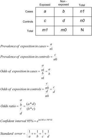
Case–control studies use the odds ratio (OR) as a measure to evaluate the strength of association between a factor (exposure) and the event (health condition or disease) under study. This measure indicates the relative frequency of exposure between cases and controls, as shown in Figure 3.2. The quotient of OR of exposure in cases and the OR of exposure in controls corresponds to the OR of exposure.
 |
| FIGURE 3.2 |
In this type of study, the incidence of disease cannot be estimated both in exposed and in nonexposed individuals because they are selected based on the presence or absence of the condition under study and not by their exposure status (with the exception of some variants of case–control studies, such as the nested case–control, the case–cohort, and the case–crossover designs). On the other hand, although relative risk is not directly calculated, when frequency of disease is low, OR is a nonbiased estimator of the incidence rate ratio or relative risk (Lazcano-Ponce et al., 2001).
Odds ratio values oscillate between 0 and infinite. The OR obtained from a case–control study indicates how many times higher (when OR is >1) or lower (when OR is <1) the probability is that cases have been exposed to a factor under study compared to controls (dos Santos-Silva, 1999a). The former are considered risk factors (i.e., increases in the likelihood of having the characteristic under study) and the latter protective factors (i.e., decreases in the likelihood of developing the phenomenon under study).
Once the OR is estimated, it is useful to calculate a measure of variability to that point estimation. The confidence interval indicates a range within which the true value of association is estimated to lie if such value would have been obtained from the total population. The confidence interval (i.e., 95%) determines how likely the interval is to contain the point estimation. If the confidence interval includes 1, the association is not statistically significant. At a given level of confidence, and all other things being equal, a result with a smaller confidence interval is more reliable than a result with a larger one. In this sense, sample size is an important determinant of the width and precision of a confidence interval in the estimation procedure. Figure 3.2 shows how to calculate these measures.
Odds ratios are commonly interpreted as a measure of casual relation between exposure and the event under study. For this to be true, some conditions are needed. Controls should be part of and be a representative sample of the same base population as cases. Most case–control studies are retrospective, and as a result, a perfect causal relation cannot always be verified because the disease/health condition is evaluated before exposure (Hernández-Ávila & López-Moreno, 2007). This situation also introduces other errors or bias (Lazcano-Ponce et al., 2001).
3.5. Subtypes of Case–Control Studies
Table 3.5 describes some of the most important variants of case–control studies in epidemiological research.
| Subtype | Characteristics |
|---|---|
| Case–cohort studies | Studies in which the source population is a cohort and every person in the cohort has an equal chance of being included in the study as a control, regardless of how much time that individual has contributed to the person-time experience of the cohort. This is a logical way to conduct a case–control study when the effect measure of interest is the ratio of incidence proportions rather than a rate ratio. Paralleling the earlier development, the average risk (or proportion) of falling ill during a specified risk period may be written. An advantage of the case–cohort design is that it allows one to conduct a set of case–controls studies from a single cohort, all of which use the same control group. Just as one can measure the incidence rate of a variety of diseases within a single cohort, one can conduct a set of simultaneous case–cohort studies using a single control group. |
| Nested case–control studies | Studies that use a risk groups sampling approach to identify cases of a disease that occur in a defined cohort and, for each, a specified number of matched controls is selected from among those in the cohort who have not developed the disease by the time of disease occurrence in the case. Sampling could be assumed as nested inside a dynamic cohort, where study subjects remain in the cohort for variable time and where exposure could take different values over time. |
| Cumulative (“epidemic”) case–control studies | Studies that are aimed at addressing a risk that ends before subject selection begins (i.e., some epidemic diseases). In such a situation, an investigator might select controls from that portion of the population that remains after eliminating the accumulated cases; that is, one selects controls from among noncases (those who remain free of disease at the end of the epidemic). |
| Case-only studies | Studies in which cases are the only subjects used to estimate or test hypotheses about effects. For example, it is sometimes possible to employ theoretical considerations to construct a prior distribution of exposure in the source population and to use this distribution in place of an observed control series. Such situations naturally arise in genetic studies, in which basic laws of inheritance may be combined with certain assumptions to derive a population- or parental-specific distribution of genotypes. It is also possible to study certain aspects of joint effects (interactions) of genetic and environmental factors without using control subjects. |
| Case–crossover studies | Studies that use one or more (predisease) time periods as matched “control periods” for the case. The exposure status of the case at the time of the disease onset is compared with the distribution of exposure status for the same individual in the earlier periods. Such a comparison depends on the assumption that neither exposure nor confounders are changing over time in a systematic way. Only a limited set of research topics are amenable to the case–crossover design. The exposure must vary over time within individuals rather than stay constant. Like the crossover study, the exposure must also have a short induction time and a transient effect; otherwise, exposures in the distant past could be the cause of a recent disease onset (the “carryover” effect). |
| Two-stage sampling | Studies in which the control series comprises a relatively large number of individuals (possible everyone in the source population), from whom exposure information or perhaps some limited amount of information on other relevant variables is obtained. Then, for a subsample of the controls (or cases), more detailed information is obtained on some variables. It is useful when it is relatively inexpensive to obtain the exposure information but the covariate information is more expensive to obtain; when exposure information has already been collected on the entire population, but covariate information is needed; and in cohort studies when more information is required than was gathered at baseline. |
| Proportional mortality studies | Studies in which cases are deaths occurring within the source population. Controls are not selected directly from the source population. This control series is acceptable if the exposure distribution within this group is similar to that of the source population. Consequently, the control series should be restricted to categories of death that are not related to the exposure. |
3.6. Problems with Case–Control Studies
3.6.1. Bias
Because case–control studies are commonly retrospective, they are particularly vulnerable to the introduction of errors in the process of selection and information gathering. For this reason, these studies are not considered to be appropriate for finding causal effects (Table 3.6; Hernández-Ávila & López-Moreno, 2007). However, in some instances, case–control studies can be prospective, increasing their potential to study causality (Hernández-Ávila & López-Moreno, 2007).
| Selection bias |
| Nonresponse |
| Information bias |
| Measurement error |
| Bias by the interviewer (observer bias) |
| Interviewee bias |
| Memory bias (recall bias) |
| Exposure bias |
| Confusion bias |
Error in the measurement of variables is unavoidable in epidemiologic studies, particularly when information is obtained retrospectively (Wacholder, et al., 1992). With nondifferential errors, the bias is typically (but not always) in a predictable direction (toward lack of association) and, unless the measurement is so bad as to be negatively correlated with the truth, seldom reverses the direction of the association. On the other hand, the effect of differential measurement error on estimates of association is usually unpredictable (Wacholder, et al., 1992).
A widespread concern about survey-based case–control studies is that cases recall previous exposures differently than do controls. Cases may spend time thinking about possible reasons for their illness, may search their memories for past exposure or even exaggerate or fabricate exposure, or may try to deny any responsibility for the disease. Therefore, some suggest using control groups of diseased subjects to achieve equal accuracy. Although accuracy of information and how that accuracy differs between cases and controls are considerations in the choice of control group, one must also be concerned about choosing controls with conditions possibly related to exposure (Wacholder, et al., 1992b). The degree of accuracy in measuring the exposure of interest for the cases should be equivalent to the degree of accuracy for the controls, unless the effect of the inaccuracy can be controlled in the analysis (comparably accuracy principle) (Wacholder, et al., 1992).
The efficiency principle can conflict with the deconfounding principle when controls are selected to have the same values of confounders as cases, thus restricting the variability of the confounding variables. This in turn reduces the precision of estimates of effect. When control of confounding is essential for bias reduction, the efficiency principle must be subordinated (Wacholder, et al., 1992). A study carried out to quantify the relationship between acute alcohol consumption and risk of injury (Watt, Purdie, Roche, & McClure, 2004), in the context of other potential confounding factors (i.e., usual alcohol intake, risk-taking behavior, and substance use, defined as use of prescription/over-the-counter medication or illicit substances), used three separate measures of alcohol consumption. A hospital-based case–control study was used in which 488 cases were matched to 488 population controls on gender, age group, neighborhood, and day and time of injury. It was concluded that acute alcohol consumption significantly increased the risk of injury, even when situational and other risk factors were considered.
It is important to note that Watt et al. (2004) did not report the effect of the mix of illnesses seen in the hospital on alcohol use or the effect of alcohol use on seeking medical care for injury or illness. Thus, the extent of over- or underestimation of alcohol’s effect on injury is uncertain. If alcohol contributes to the problem presented by the control patients or to the probability of seeking medical attention, the difference in alcohol measured between cases and controls could be less than if persons exposed to the circumstances of injury who had no reason to seek medical attention were chosen as controls. If the medical condition is such that the control patients would not have been engaged in activities similar to those of the injured people, the effect of aspects of those activities would be overestimated (Robertson, 1992).
In addition, the relationship between alcohol and injury appears to be confounded in Watt et al.’s (2004) study by usual drinking patterns, risk-taking behavior, and substance use. One way of studying the factors would be to replicate these case–control studies and measure hypothesized biological factors that might contribute to alcohol use, other behaviors, or both jointly. Two major problems would be encountered in such a study. First, although measurement of alcohol in breath samples of controls is seldom resisted by persons selected as controls, requests for blood or other biological specimens might not be acceptable. Second, reliable evidence that trauma does not change the hypothesized biological factor is necessary before assuming that a difference between cases and controls is indicative of causation (Robertson, 1992). For example, research was done to measure state anger and the risk of injury where cases were patients seeking care for an acute injury. They were compared with two controls: the patient himself or herself 24h earlier and an individual recruited by telephone from the community and matched for age group, sex, and time. Self-reported anger was assessed with three Likert scale items. Anger just before the injury was compared in case–crossover analyses with the respondent’s own level of anger 24h earlier and, as in case–control analyses, with community participants’ level of anger at the same hour of the same day of the week during a subsequent week. Anger was not associated with fall and traffic injuries, but anger was strongly associated with intentional injuries inflicted by another person in both men and women (Vinson & Arelli, 2006).
3.6.2. Is Representativeness a Problem in Case–Control Studies?
Although much emphasis has been given to the necessity that selected cases should be representative of all cases, as noted by Rothman and Greenland (1998), such advice can be misleading, given that sometimes cases (and thus controls) may be restricted to any type of case that may be of interest for research. Studies may focus only on women or only on the most severe cases or even specific groups of a population (elderly, schoolchildren, etc.). In this sense, case definition will implicitly define the source population for cases, from which the controls should be drawn. It is this source of population for the cases that the controls should represent, not the entire nondiseased population. Achieving representativeness in this context would be neither easy nor desirable, and a perfectly valid case–control study would be possible (Rothman & Greenland, 1998).
The study base principle entails the requirement of representativeness of the base but not necessarily of the general population. Representativeness of the general population is crucial in estimating the prevalence of disease, the attributable risk, or the distribution of a variable in a population based on a sample. However, representativeness per se is not needed in analytical studies of the relation between an exposure and disease. An association found in any subpopulation may be of interest in itself; in a representative population, an association that is limited to one group may be obscured because the effect is weaker in other groups or because of differences in the distribution of the exposure. On the other hand, detection of variability of the strength of association (effect modification) can be missed if the study base is narrowly defined. If there is reason to believe that an effect is strongest in one particular subgroup, exclusion of other subgroups might be the best strategy for demonstrating that effect; thus, a study of the effect of a possible risk factor for myocardial infarction might restrict the base to subjects who had a previous one (Wacholder, et al., 1992).
3.7. Advantages and Disadvantages of Case–Control Studies
Table 3.7 highlights the most important advantages and disadvantages of case–control designs that should be taken into account when determining which type of epidemiological approach to use.
| Advantage | Disadvantage |
|---|---|
| For diseases that are sufficiently rare, case–control studies are an efficient and useful alternative (Lazcano-Ponce et al., 2001 and Rothman and Greenland, 1998). This is also the case for diseases with prolonged latency periods (dos Santos-Silva, 1999a, Hernández-Ávila and López-Moreno, 2007 and Lazcano-Ponce et al., 2001). | For exposures that are extremely rare, case–control studies are not efficient (Rothman & Greenland, 1998) unless exposition is responsible for a large proportion of cases (high population attributable fraction) (dos Santos-Silva, 1999a). |
| Relatively easy to perform (Rothman & Greenland, 1998). | Sometimes it is difficult to define the base population from which cases are drawn (Hernández-Ávila & López-Moreno, 2007). |
| Not extremely expensive nor time-consuming, especially compared to cohort studies (dos Santos-Silva, 1999a, Hernández-Ávila and López-Moreno, 2007 and Rothman and Greenland, 1998). | Given that exposure is measured, quantified, or reconstructed retrospectively in most of the cases, information bias is common (Lazcano-Ponce et al., 2001). This is sometimes due to problems in precise measurement of exposition levels (exposure bias) (dos Santos-Silva, 1999a and Hernández-Ávila and López-Moreno, 2007). |
| Require fewer subjects under study than other epidemiological study designs. For example, prospective cohort studies would require the inclusion of a larger number of individuals and a longer follow-up period to ensure the inclusion of a sufficient number of cases (dos Santos-Silva, 1999a). | Selection bias is common (dos Santos-Silva, 1999a, Hernández-Ávila and López-Moreno, 2007 and Lazcano-Ponce et al., 2001). There are a variety of reasons for this, including the following: • Difficulty of finding an adequate control group • If exposure of interest determines selection of cases and controls in a different manner (diagnostic bias) |
| Several expositions or risk factors of the disease or health condition under study can be analyzed at the same time (dos Santos-Silva, 1999a, Hernández-Ávila and López-Moreno, 2007 and Lazcano-Ponce et al., 2001). | It is not possible to directly estimate incidence or prevalence for both exposed and nonexposed (Hernández-Ávila & López-Moreno, 2007). |
| Allows the estimation of true relative risk if and when representativeness, simultaneity, and homogeneity assumptions are met (Lazcano-Ponce et al., 2001). | Temporality between exposure and disease could be difficult to establish (reverse causality) (dos Santos-Silva, 1999a and Hernández-Ávila and López-Moreno, 2007). |
| Lack of representativeness (except when the study is population based) (dos Santos-Silva, 1999a). | |
| Not useful when disease under study is measured continuously (Lazcano-Ponce et al., 2001). | |
| If condition of interest is highly prevalent (more than 5%), the odds ratio is not a confident estimation of risk ratio (Lazcano-Ponce et al., 2001). |
4. Conclusions
Throughout the world, no matter the level of motorization, there is a need to improve road safety for all road actors to reduce current inequalities and the risk of road traffic injuries. Road safety efforts must be evidence based, fully funded, properly resourced, and sustainable. The best way to achieve this is through research that requires an approach that includes various key elements such as policy makers, decision makers, professionals, and practitioners who recognize that the traffic injury problem is an urgent one but one for which solutions are already largely known. It will require that road safety strategies be integrated with other strategic, and sometimes competing, goals, such as those relating to the environment and to accessibility and mobility.
Among the many research-related needs for road injury prevention, it is necessary to encourage the development of professional expertise across a range of disciplines at the national level along with regional cooperation and exchange of information to achieve maximum benefit. Developing such expertise should be a priority where it does not exist. This chapter sufficiently clarifies the advantages and limitations of using case–control designs. They are important for researching the causes of road traffic injuries and for determining the following:
References
Ameratunga, S.; Hijar, M.; Norton, R., Road-traffic injuries: Confronting disparities to address a global-health problem, Lancet 367 (9521) (2006) 1533–1540.
Celis, A.; Gomez, Z.; Martinez-Sotomayor, A.; Arcila, L.; Villasenor, M., Family characteristics and pedestrian injury risk in Mexican children, Injury Prevention 9 (1) (2003) 58–61.
dos Santos-Silva, I., Estudios caso–control, In: Epidemiología del cáncer: Principios y métodos (1999) Agencia Internacional de Investigación sobre el Cáncer, Lyon, France, pp. 199–224.
dos Santos-Silva, I., Revisión de los diseños de estudios, In: Epidemiología del cáncer: Principios y métodos (1999) Agencia Internacional de Investigación sobre el Cáncer, Lyon, France, pp. 89–108.
European Road Safety Action Programme, Halving the number of road accident victims in the European Union by 2010: A shared responsibility. (2003) Commission of the European Communities, Brussels.
Fontaine, H.; Gourlet, Y., Fatal pedestrian accidents in France: A typological analysis, Accident Analysis and Prevention 29 (3) (1997) 303–312.
Haddon Jr., W.; Valien, P.; McCarroll, J.R.; Umberger, C.J., A controlled investigation of the characteristics of adult pedestrians fatally injured by motor vehicles in Manhattan, Journal of Chronic Diseases 14 (1961) 655–678.
Hernandez-Avila, M.; Garrido, F.; Salazar-Martinez, E., Biases in epidemiological studies, Salud Publica de Mexico 42 (5) (2000) 438–446.
Hernández-Ávila, M.; López-Moreno, S., Diseño de estudios epidemiológicos, In: (Editor: Hernández-Ávila, M.) Epidemiología. Diseño y análisis de estudios (2007) Instituto Nacional de Salud Pública / Editorial Médica Panamericana S.A. de C.V, Cuernavaca, Morelos, México, pp. 17–32.
Híjar-Medina, M.C.; Flores-Aldana, M.E.; Lopez-Lopez, M.V., Safety belt use and severity of injuries in traffic accidents, Salud Publica Mex 38 (2) (1996) 118–127.
Híjar-Medina, M.C.; Vázquez-Vela, E., Foro nacional sobre accidentes de tránsito en México. Enfrentando los retos a través de una visión intersectorial, In: (Editor: Primera) (2003) Instituto Nacional de Salud Pública, Cuernavaca, Morelos, México.
Impacts Monitoring Group in the Congestion Charging Division of Transport for London, Impacts monitoring first annual report. (2003) Transport for London, London.
Jones, C.; Harvey, A.G.; Brewin, C.R., Traumatic brain injury, dissociation, and posttraumatic stress disorder in road traffic accident survivors, Journal of Traumatic Stress 18 (3) (2005) 181–191.
Khayesi, M., Liveable streets for pedestrians in Nairobi: The challenge of road traffic accidents, In: (Editors: Whitelegg, J.; Haq, G.) The Earthscan reader on world transport policy and practice (2003) Earthscan, London, pp. 35–41.
Koepsell, T.; McCloskey, L.; Wolf, M.; Moudon, A.V.; Buchner, D.; Kraus, J.; et al., Crosswalk markings and the risk of pedestrian–motor vehicle collisions in older pedestrians, Journal of the American Medical Association 288 (17) (2002) 2136–2143.
Kraus, J.F.; Hooten, E.G.; Brown, K.A.; Peek-Asa, C.; Heye, C.; McArthur, D.L., Child pedestrian and bicyclist injuries: Results of community surveillance and a case–control study, Injury Prevention 2 (3) (1996) 212–218.
Lazcano-Ponce, E.; Salazar-Martinez, E.; Hernandez-Avila, M., Case–control epidemiological studies: Theoretical bases, variants and applications, Salud Publica de Mexico 43 (2) (2001) 135–150.
Lightstone, A.S.; Peek-Asa, C.; Kraus, J.F., Relationship between driver’s record and automobile versus child pedestrian collisions, Injury Prevention 3 (4) (1997) 262–266.
Mayou, R.; Bryant, B., Consequences of road traffic accidents for different types of road user, Injury 34 (3) (2003) 197–202.
In: (Editors: Peden, M.; Scurfield, R.; Sleet, D.; Mohan, D.; Hyder, A.; Jarawan, E.; et al.) World report on road traffic injury prevention (2004) World Health Organisation, Geneva.
Razzak, J.A.; Luby, S.P., Estimating deaths and injuries due to road traffic accidents in Karachi, Pakistan, through the capture–recapture method, International Journal of Epidemiology 27 (5) (1998) 866–870.
Roberts, I.; Norton, R., Sensory deficit and the risk of pedestrian injury, Injury Prevention 1 (1) (1995) 12–14.
Robertson, L.S., Injury epidemiology. (1992) Oxford University Press, New York.
Rothman, K.J.; Greenland, S., Modern epidemiology. 2nd ed. (1998) Lippincott-Raven, Philadelphia.
Stevenson, M.; Jamrozik, K.; Burton, P., A case–control study of childhood pedestrian injuries in Perth, Western Australia, Journal of Epidemiology and Community Health 50 (3) (1996) 280–287.
Tester, J.M.; Rutherford, G.W.; Wald, Z.; Rutherford, M.W., A matched case–control study evaluating the effectiveness of speed humps in reducing child pedestrian injuries, American Journal of Public Health 94 (4) (2004) 646–650.
Tingvall, C., The zero vision, In: (Editors: van Holst, H.; Nygren, A.; Thord, R.) Transportation, traffic safety and health: The new mobility8th ed. (1997) Springer-Verlag, Berlin, pp. 35–57.
Vinson, D.C.; Arelli, V., State anger and the risk of injury: A case–control and case–crossover study, Annals of Family Medicine 4 (1) (2006) 63–68.
Vinson, D.C.; Maclure, M.; Reidinger, C.; Smith, G.S., A population-based case–crossover and case–control study of alcohol and the risk of injury, Journal of Studies on Alcohol 64 (3) (2003) 358–366.
von Kries, R.; Kohne, C.; Bohm, O.; von Voss, H., Road injuries in school age children: Relation to environmental factors amenable to interventions, Injury Prevention 4 (2) (1998) 103–105.
Wacholder, S.; McLaughlin, J.K.; Silverman, D.T.; Mandel, J.S., Selection of controls in case–control studies: I. Principles, American Journal of Epidemiology 135 (9) (1992) 1019–1028.
Wacholder, S.; Silverman, D.T.; McLaughlin, J.K.; Mandel, J.S., Selection of controls in case–control studies: II. Types of controls, American Journal of Epidemiology 135 (9) (1992) 1029–1041.
Wacholder, S.; Silverman, D.T.; McLaughlin, J.K.; Mandel, J.S., Selection of controls in case-control studies: III. Design options, American Journal of Epidemiology 135 (9) (1992) 1042–1050.
Wang, S.Y.; Chi, G.B.; Jing, C.X.; Dong, X.M.; Wu, C.P.; Li, L.P., Trends in road traffic crashes and associated injury and fatality in the People’s Republic of China, 1951–1999, Injury Control and Safety Promotion 10 (1–2) (2003) 83–87.
Watt, K.; Purdie, D.M.; Roche, A.M.; McClure, R.J., Risk of injury from acute alcohol consumption and the influence of confounders, Addiction 99 (10) (2004) 1262–1273.
Wells, S.; Mullin, B.; Norton, R.; Langley, J.; Connor, J.; Lay-Yee, R.; et al., Motorcycle rider conspicuity and crash related injury: Case–control study, British Medical Journal 328 (7444) (2004) 857.
Wintemute, G.J.; Kraus, J.F.; Teret, S.P.; Wright, M.A., Death resulting from motor vehicle immersions: The nature of the injuries, personal and environmental contributing factors, and potential interventions, American Journal of Public Health 80 (9) (1990) 1068–1070.
Yu, J.M.; Wang, Y.C.; Chen, F., A case–control study on road-related traffic injury in Shanghai, Zhonghua Liu Xing Bing Xue Za Zhi 26 (5) (2005) 344–347.