Chapter 6

Solving Linear Equations

In This Chapter

Simplifying equations before applying rules

Isolating variables on one side of the equation

Using proportions to solve equations

Adapting formulas for easier use

Linear equations consist of some terms that have variables and others that are constants. A standard form of a linear equation is ax + b = c. What distinguishes linear equations from the rest of the pack is the fact that the variables are always raised to the first power.

In this chapter, I take you through many different types of opportunities for dealing with linear equations. Most of the principles you use with these first-degree equations are applicable to the higher-order equations, so you don’t have to start from scratch later on.

Playing by the Rules

When you’re solving equations with just two terms or three terms or even more than three terms, the big question is: “What do I do first?”

Actually, as long as the equation stays balanced, you can perform any operations in any order. But you also don’t want to waste your time performing operations that don’t get you anywhere or even make matters worse.

The following list tells you how to solve your equations in the best order. The basic process behind solving equations is to use the reverse of the order of operations.

The order of operations (see Chapter 3) is powers or roots first, then multiplication and division, and addition and subtraction last. Grouping symbols override the order — you perform the operations inside the grouping symbols to get rid of them first.

When you’re solving equations, you still usually deal with the grouping symbols first, but, for the rest of the equation, you reverse the order of operations:

1. Do all the addition and subtraction.

Combine all terms that can be combined both on the same side of the equation and on opposite sides using addition and subtraction.

2. Do all multiplication and division.

This step is usually the one that isolates or solves for the value of the variable or some power of the variable.

3. Multiply exponents and find the roots.

Powers and roots aren’t found in these linear equations — they come in quadratic and higher-powered equations. But these would come next in the reverse order of operations.

When solving linear equations, the goal is to isolate the variable you’re trying to find the value of. Isolating it, or getting it all alone on one side, can take one step or many steps. And it has to be done according to the rules.

Solving Equations with Two Terms

Linear equations contain variables raised to the first power. The easiest types of linear equations to solve are those consisting of two terms, such as those in the form: ax = b or cx + d = 0.

Linear equations that contain just two terms are solved with multiplication, division, reciprocals, or some combinations of the operations.

Depending on division

One of the most basic methods for solving equations is to divide each side of the equation by the same number. Many formulas and equations include a coefficient (multiplier) with the variable. To get rid of the coefficient and solve the equation, you divide. The following example takes you step-by-step through solving with division.

Solve for x in 20x = 170.

1. Determine the coefficient of the variable and divide both sides by it.

Because the equation involves multiplying by 20, undo the multiplication in the equation by doing the opposite, which is division. Divide each side by 20:

2. Reduce both sides of the equal sign.

Now, let me show you an example with a practical application embedded in it.

You need to buy 300 doughnuts for a big meeting. How many dozen doughnuts is that?

Let d represent the number of dozen doughnuts you need. There are 12 doughnuts in a dozen, so 12d = 300. Twelve times the number of dozens of doughnuts you need has to equal 300.

1. Determine the coefficient of the variable and divide both sides by it.

Divide each side by 12.

2. Reduce both sides of the equal sign.

d = 25 dozen donuts

Making use of multiplication

The opposite operation of multiplication is division. I use division in the preceding section to solve equations where a number multiplies the variable. The reverse occurs in this section: I use multiplication where a number already divides the variable. The first example walks you through the steps needed.

Solve for y in .

1. Determine the value that divides the variable and multiply both sides by it.

In this case, 11 is dividing the y, so that’s what you multiply by.

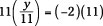
2. Reduce on the left side and multiply on the right.

Next, look at an example that’s applicable — a bit hairy (pardon the pun), but you read about situations like this all the time.

A wealthy woman’s will dictated that her fortune be divided evenly among her nine cats. Each feline got $500,000, so what was her total fortune before it was split up? (Cats don’t pay inheritance tax. Does that give you paws? Ouch.)

Let f represent the amount of her fortune. Then you can write the equation:

In other words, the fortune divided by 9 gave a share of $500,000.

1. Determine the value that divides the variable and multiply both sides by it.

In this equation, the fortune was divided. Solve the puzzle by multiplying each side by 9. The opposite of division is multiplication, so multiplication undoes what division did.

2. Reduce on the left and multiply on the right.

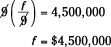
Her fortune was $4.5 million! Those are nine very happy kitties. You can bet their caretakers hope they have nice, long lives.

In the next example, the variable is multiplied by 4 and divided by 5. So, you solve the problem using both multiplication and division.

Solve for a in .

1. Determine what is dividing the variable.

In this case, the 5 is dividing both the 4 and the variable a.

2. Multiply the values on each side of the equal sign by 5.

3. Reduce and simplify.

4. Determine what is multiplying the variable.

The number 4 is the coefficient and multiplies the a.

5. Divide the values on each side of the equal sign.

6. Reduce and simplify.

A simpler way of solving this last equation is to multiply by the reciprocal of the variable’s coefficient. I show you that alternative next.

Reciprocating the invitation

The reciprocal of a number is its “flip.” A more mathematical definition is that a number and its reciprocal have a product of 1.

What makes the reciprocal so important in algebra is that you can create the number 1 as a coefficient of a variable by multiplying by the reciprocal of the current coefficient. So, in a way, this process is just a special case of multiplying each side by the same number.

In the following example, I solve a problem (the last example in the preceding section) using the reciprocal instead of doing the two operations of multiplication and division.

Solve for a in .

The coefficient of the variable a is the fraction . The

reciprocal of is . So, to solve for a, you multiply each

side of the equation by :

Taking on Three Terms

The standard form of a linear equation is ax + b = c. In the “Solving Equations with Two Terms” section, earlier in this chapter, you have linear equations for which the value of b is 0, which gives you just ax = c. In this section, I introduce that extra constant value and show you how to deal with it. Also, in this section, you find equations that start out with more than one variable term, and you work toward combining and creating a new equation with just the one variable.

In general, you solve linear equations by simplifying and performing operations that give you a variable term on one side of the equal sign and a constant term on the other side. Then you can use multiplication or division to finish the problem.

Eliminating a constant term

When you have a linear equation involving three terms, and just one of the terms contains a variable factor, you add or subtract a constant to isolate that variable term — get it by itself on one side of the equation.

Solve for y in 3y – 11 = 19.

To isolate the y term, you add 11 to each side of the equation. The number 11 is chosen, because it’s the opposite of –11, and the sum of –11 and 11 is 0.

Now you have a linear equation in two terms, which is solved by dividing each side of the equation by 3:

Vanquishing the extra variable term

One aim of the linear-equation solver is to get the variable term on one side of the equation and the constant term on the other side. In the preceding section, I show you how to get rid of the pesky extra constant. But what if you have more than one variable term? Can that be dealt with as easily as the constant numbers? The answer is a resounding “yes.”

To reduce your linear equation to one variable term, you first perform any addition or subtraction necessary to get all the variable terms on one side of the equation.

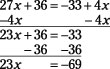
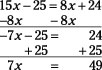
Solve for the value of x in 5x – 4 = 3x + 8.

First, subtract 3x from each side of the equation. That step removes the x term from the right side. Subtracting 5x – 3x, you get 2x, because the two terms have the same variable:

Now the problem looks like those from the previous section. I isolate the variable term by adding 4 to each side of the equation:

Now the problem is finished by dividing each side of the equation by 2:

Breaking Up the Groups

Linear equations don’t always start out in the nice, ax + b = c form. Sometimes, because of the complexity of the application, a linear equation can contain multiple variable and constant terms and lots of grouping symbols, such as in this equation:

3[4x + 5(x + 2)] + 6 = 1 – 2[9 – 2(x – 4)]

The different types of grouping symbols are used for nested expressions (one inside the other). The rules regarding order of operations (see Chapter 3) apply as you work toward figuring out what the variable x represents.

Nesting isn’t for the birds

When you have a number or variable that needs to be multiplied by every value inside parentheses, brackets, braces, or a combination of those grouping symbols, you distribute that number or variable. Distributing means that the number or variable next to the grouping symbol multiplies every value inside the grouping symbol. If two or more of the grouping symbols are inside one another, they’re nested. Nested expressions are written within parentheses, brackets, and braces to make the intent clearer.

Distributing first

Equations containing grouping symbols offer opportunities for making wise decisions. In some cases you need to distribute, working from the inside out, and in other cases it’s wise to multiply or divide first. In general, you’ll distribute first if you find more than two terms in the entire equation.

Solve for x in 3[4x + 5(x + 2)] + 6 = 1 – 2[9 – 2(x – 4)].

The best way to sort through all these operations is to simplify from the inside out. You see parentheses within brackets. The binomials in the parentheses have multipliers. I’ll step through this carefully to show you an organized plan of attack.

First, distribute the 5 over the binomial inside the left parentheses and the –2 over the binomial inside the right parentheses:

3[4x + 5x + 10] + 6 = 1 – 2[9 – 2x + 8]

Now combine terms within the brackets:

3[9x + 10] + 6 = 1 – 2[17 – 2x]

Distribute the 3 over the two terms in the left brackets and the –2 over the terms in the right brackets:

27x + 30 + 6 = 1 – 34 + 4x

The constant terms on each side can be combined:

27x + 36 = –33 + 4x

Now subtract 4x from each side and subtract 36 from each side:

Now, dividing each side of the equation by 23, you get that x = –3.

Multiplying before distributing

In this section, I show you where it might be easier to divide through by a number rather than distribute first. My only caution is that you always divide (or multiply) each term by the same number.

This example mixes two different situations that are actually the same. The terms in the equation either have a fractional multiplier or are in a fraction themselves. The point of the example is to show when multiplying each term by the same number first is preferable to distributing first.

Solve for x in the following equation:

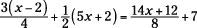
At first glance, the equation looks a bit forbidding. But quick action — in the form of multiplying each term by 8 — takes care of all the fractions. You’re left with rather large numbers, but that’s still nicer than fractions with different denominators. I choose to multiply by 8, because that’s the least common denominator of each term (even the last term). Each of the four terms is multiplied by 8:

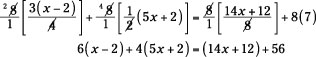
Do the multiplication and distributing in steps to avoid errors:

6x – 12 + 20x + 8 = 14x + 12 + 56

The two variable terms on the left and the two constant terms on the left can be combined. Likewise, combine the two constant terms on the right:

26x – 4 = 14x + 68

Now subtract 14x from each side and add 4 to each side:

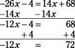
Dividing each side of the equation by 12, you see that x = 6.

Focusing on Fractions

Fractions appear frequently in algebraic equations. In the “Multiplying before distributing” section, earlier in this chapter, I show you how to remove the fractions from an equation when you have the right situation. In this section, I show you how to leave in the fraction, take advantage of the fractional setup, and use it to your advantage.

Promoting proportions

A proportion is an equation. It consist of two ratios (fractions)

set equal to one another. When you write , you’re

writing a proportion. Before I show you how proportions are solved in algebra problems, I have some properties to share.

Given the proportion :

The cross-products are equal: ad = bc.

The reciprocals are equal: .

You can reduce the fractions vertically, as usual: .

You can reduce horizontally, across the equal sign:

or .

Now I’ll use some of the properties of proportions to solve equations.

Solve for x: .

Before cross-multiplying, reduce the fraction on the right by dividing the numerator and denominator by 3:

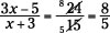
Now, using the cross-multiplying rule:

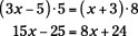
Subtract 8x from each side, and add 25 to each side:

Finally, divide each side by 7, and you get x = 7.

When reducing proportions, you can divide vertically or horizontally, but you can’t reduce the fractions diagonally. The diagonal reductions are done when you’re multiplying fractions and you have a multiplication symbol between them, not an equal sign between them.

Taking advantage of proportions

Proportions are very nice to work with because of their unique properties of reducing and changing into non-fractional equations. Many equations involving fractions must be dealt with in that fractional form, but other equations are easily changed into proportions. When possible, you want to take advantage of the situations where transformations can be done.

Solve the following equation for x:

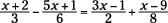
You could solve the problem by multiplying each fraction by the least common factor of all the fractions: 24.

Another option is to find a common denominator for the two fractions on the left and subtract them, and then find a common denominator for the two fractions on the right and add them. Your result is a proportion:

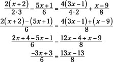
The proportion can be reduced by dividing by 2 horizontally:

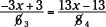
Now cross-multiply and simplify the products:

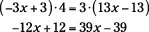
Add 12x to each side, and then add 39 to each side:

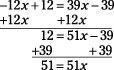
The last step consists of just dividing each side by 51 to get 1 = x.

Changing Formulas by Solving for Variables

A formula is an equation that represents a relationship between some structures, quantities, or other entities. It’s a rule that uses mathematical computations and can be counted on to be accurate each time you use it (when applied correctly).

Here are some of the more commonly used formulas that contain only variables raised to the first power:

: The area of triangle involves base and height.

I = Prt: The interest earned uses principal, rate, and time.

C = 2πr: Circumference is twice π times the radius.

: Degrees Fahrenheit can be expressed in

terms of degrees Celsius.

P = R – C: Profit is based on revenue and cost.

When you use a formula to find the indicated variable (the one on the left of the equal sign), then you just put the numbers in, and out pops the answer. Sometimes, though, you’re looking for one of the other variables in the equation and end up solving for that variable over and over.

For example, let’s say that you’re planning a circular rose garden in your backyard. You find edging on sale and can buy a 20-foot roll of edging, a 36-foot roll, a 40-foot roll, or a 48-foot roll. You’re going to use every bit of the edging and let the length of the roll dictate how large the garden will be. If you want to know the radius of the garden based on the length of the roll of edging, you use the formula for circumference and solve the following four equations:

20 = 2πr 36 = 2πr 40 = 2πr 48 = 2πr

Another alternative to solving four different equations is to solve for r in the formula and then put the different roll sizes into the new formula. Starting with C = 2πr, you divide each side of the equation by 2π, giving you:

The computations are much easier if you just divide the length of the roll by 2π.

Following is an example of solving for one of the variables in an equation. I won’t try to come up with any more gardening or other clever scenarios.

Solve for w in the formula for the perimeter of a rectangle: P = 2(l + w).

First, divide each side of the equation by 2 (instead of distributing the 2 through the terms in the binomial):

Now subtract l from each side. You can write the two terms as a single fraction if you want:

or