Getting Started
Keywords
Mathematica; Beginning users; 3D printing
1.1 Introduction to Mathematica
Mathematica, first released in 1988 by Wolfram Research, Inc.,
is a system for doing mathematics on a computer. Mathematica combines symbolic manipulation, numerical mathematics, outstanding graphics, and a sophisticated programming language. Because of its versatility, Mathematica has established itself as the computer algebra system of choice for many computer users. Among the over 1,000,000 users of Mathematica, 28% are engineers, 21% are computer scientists, 20% are physical scientists, 12% are mathematical scientists, and 12% are business, social, and life scientists. Two-thirds of the users are in industry and government with a small (8%) but growing number of student users. However, due to its special nature and sophistication, beginning users need to be aware of the special syntax required to make Mathematica perform in the way intended. You will find that calculations and sequences of calculations most frequently used by beginning users are discussed in detail along with many typical examples. In addition, the comprehensive index not only lists a variety of topics but also cross-references commands with frequently used options. Mathematica By Example serves as a valuable tool and reference to the beginning user of Mathematica as well as to the more sophisticated user, with specialized needs.
For information, including purchasing information, about Mathematica contact:
Corporate Headquarters:
Wolfram Research, Inc.
100 Trade Center Drive
Champaign, IL 61820
USA
telephone: 217-398-0700
fax: 217-398-0747
email: info@wolfram.com
web: http://www.wolfram.com
Europe:
Wolfram Research Europe Ltd.
10 Blenheim Office Park
Lower Road, Long Hanborough
Oxfordshire OX8 8LN
United Kingdom
telephone: +44-(0) 1993-883400
fax: +44-(0) 1993-883800
email: info-europe@wolfram.com
Asia:
Wolfram Research Asia Ltd.
Izumi Building 8F
3-2-15 Misaki-cho
Chiyoda-ku, Tokyo 101
Japan
telephone: +81-(0)3-5276-0506
fax: +81-(0)3-5276-0509
email: info-asia@wolfram.com
A Note Regarding Different Versions of Mathematica
With the release of Version 10.4 of Mathematica, many new functions and features have been added to Mathematica. We encourage users of earlier versions of Mathematica to update to Version 11 as soon as they can. All examples in Mathematica By Example, fifth edition, were completed with Version 11. In most cases, the same results will be obtained if you are using Version 10.4 or later, although the appearance of your results will almost certainly differ from that presented here. However, particular features of Version 10.4 are used and in those cases, of course, these features are not available in earlier versions. If you are using an earlier or later version of Mathematica, your results may not appear in a form identical to those found in this book: some commands found in Version 11 are not available in earlier versions of Mathematica; in later versions some commands will certainly be changed, new commands added, and obsolete commands removed. For details regarding these changes, please refer to the Documentation Center. You can determine the version of Mathematica you are using during a given Mathematica session by entering either the command $Version or the command $VersionNumber. In this text, we assume that Mathematica has been correctly installed on the computer you are using. If you need to install Mathematica on your computer, please refer to the documentation that came with the Mathematica software package.
On-line help for upgrading older versions of Mathematica and installing new versions of Mathematica is available at the Wolfram Research, Inc. website:
Details regarding what is different in Mathematica 11 from previous versions of Mathematica can be found at
http://www.wolfram.com/mathematica/new-in-11/?source=frontpage-stripe.

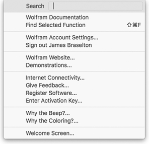
Also, when you go to the Wolfram Documentation center (under Help in the Mathematica menu) you can choose Wolfram Documentation to see the major differences. Also, the upper right hand corner of the main help page for each function will tell you if it is new in Version 11 or has been updated in Version 11.
1.1.1 Getting Started with Mathematica
We begin by introducing the essentials of Mathematica. The examples presented are taken from algebra, trigonometry, and calculus topics that most readers are familiar with to assist you in becoming acquainted with the Mathematica computer algebra system.
We assume that Mathematica has been correctly installed on the computer you are using. If you need to install Mathematica on your computer, please refer to the documentation that came with the Mathematica software package.
Start Mathematica on your computer system. Using Windows or Macintosh mouse or keyboard commands, start the Mathematica program by selecting the Mathematica icon or an existing Mathematica document (or notebook), and then clicking, double-clicking or right-clicking and selecting Open on the icon.

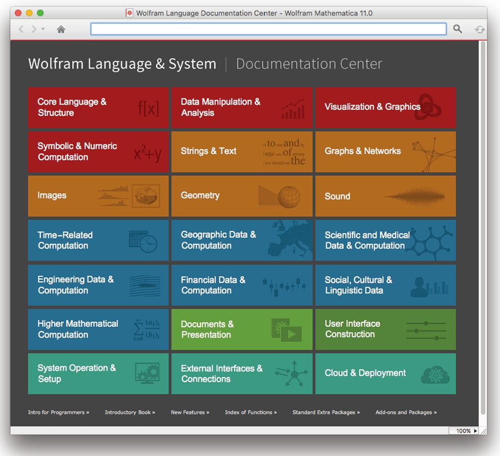
If you start Mathematica by selecting the Mathematica icon, Mathematica's startup window, “welcome screen,” is displayed, as illustrated in the following screen shot.
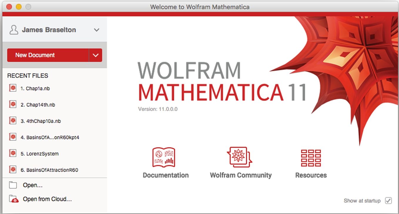
From the startup window, you can perform a variety of actions such as creating a new notebook. For example, selecting New Document generates a new Mathematica notebook.

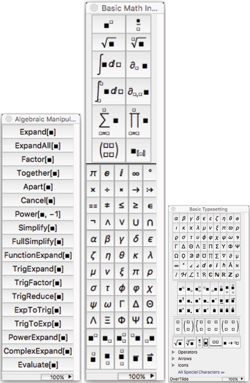
Mathematica's online help facilities are spectacular. For beginning users, one of the more convenient features are the various Palettes that are available. The Palettes provide a variety of fill-in-the blank templates to perform a wide variety of action. To access a Palette go to the Mathematica menu, select Palettes and then select a given Palette. The following screen shots show the Basic Math Assistant and Classroom Assistant palettes.

If you go further into the submenu and select Other..., you will find the Algebraic Manipulation palette, a slightly different Basic Math Input palette from that mentioned above, and the Basic Typesetting palette.
When you start typing in the new notebook created above, the thin black horizontal line near the top of the window is replaced by what you type.
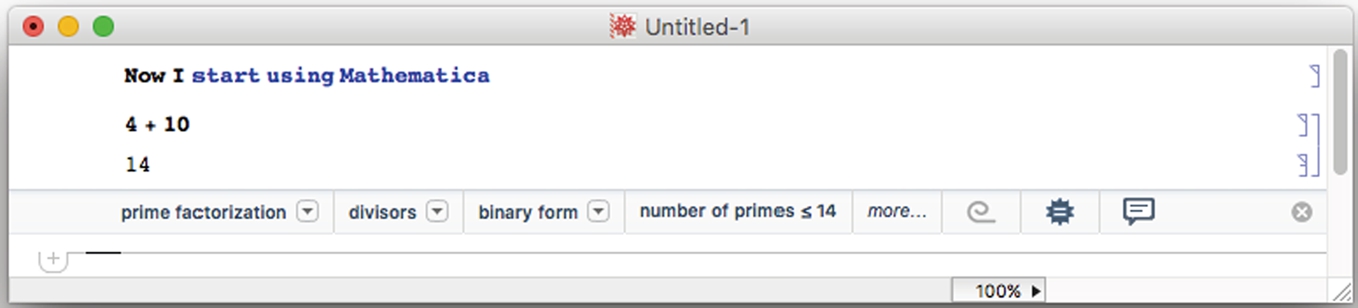
Once Mathematica has been started, computations can be carried out immediately. Mathematica commands are typed and the black horizontal line is replaced by the command, which is then evaluated by pressing Enter. Note that pressing Enter or Shift-Return evaluates commands and pressing Return yields a new line. Output is displayed below input. We illustrate some of the typical steps involved in working with Mathematica in the calculations that follow. In each case, we type the command and press Enter. Mathematica evaluates the command, displays the result, and inserts a new horizontal line after the result. For example, typing N[, then pressing the π key on the Basic Math Input palette, followed by typing ,50] and pressing the enter key
The Basic MathInput palette:

![]()
3.1415926535897932384626433832795028841971693993751
returns a 50-digit approximation of π. Note that both π and Pi represent the mathematical constant π so entering N[Pi,50] returns the same result. For basic computations, enter them into Mathematica in the same way as you would with most scientific calculators.
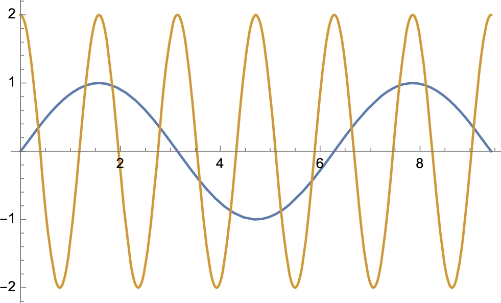
The next calculation can then be typed and entered in the same manner as the first. For example, entering
![]()
graphs the functions ![]() and
and ![]() and on the interval
and on the interval ![]() shown in Fig. 1.1.
shown in Fig. 1.1.
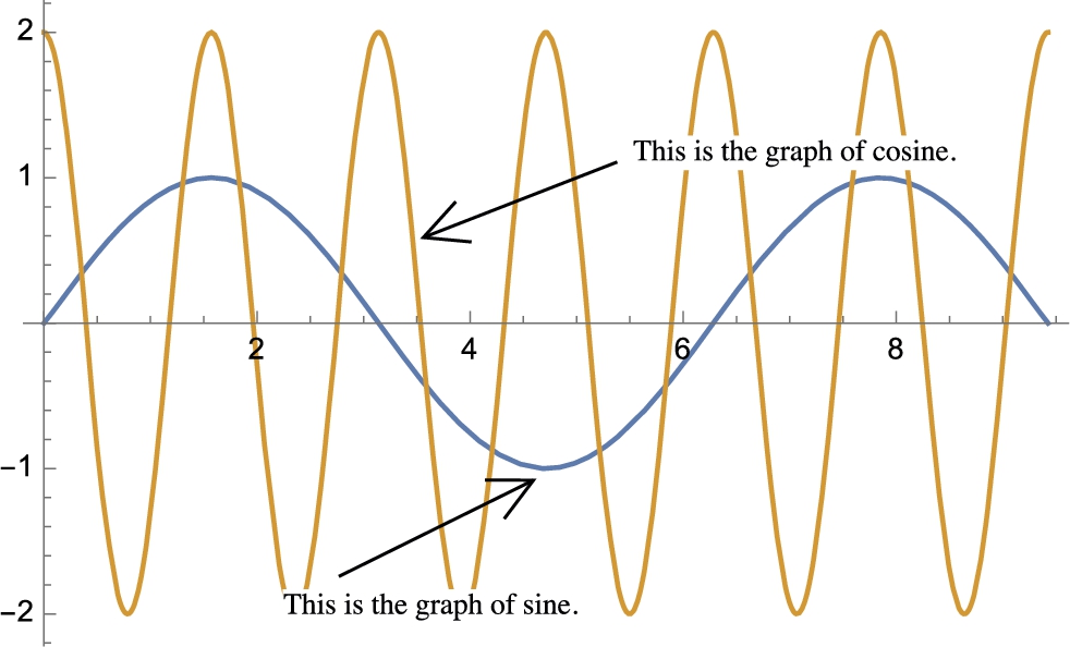
With Mathematica 11, you can easily add explanation to the graphic, by going to Graphics in the main menu, followed by Drawings Tools. Alternatively, select a graphic by clicking on it and then typing the command strokes ctrl-t to call the Drawing Tools palette. You can use the Drawing Tools palette

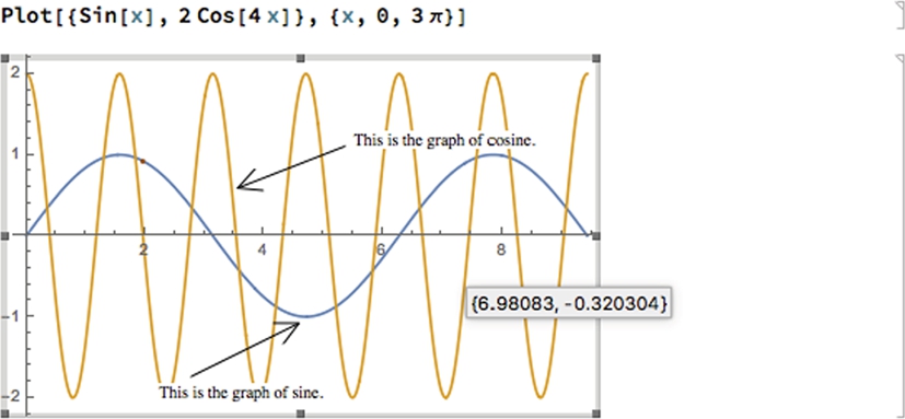
to quickly enhance a graphic. In this case we use the arrow button and “T” (text) button twice to identify each curve shown in Fig. 1.2.
The various elements can be modified by clicking on them and moving and/or typing as needed. In particular, notice the “cross-hair” button in the second row.
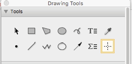
Use this button to identify coordinates in a plot. After selecting the graphic, selecting the button, then moving the cursor within the graphic will show you the coordinates.
With Mathematica 11, you can use Manipulate to illustrate how changing various parameters affect a given function or functions. With the following command we illustrate how a and b affect the period of sine and cosine and c affects the amplitude of the cosine function.
![]()
![]()
![]()
![]()

Use the slide bars to adjust the values of the parameters or click on the + button to expand the options to enter values explicitly or generate an animation to illustrate how changing the parameter values changes the problem.

Use Plot3D to generate basic three-dimensional plots. Entering
![]()
![]()
graphs the function ![]() for
for ![]() ,
, ![]() . Later we will learn other ways of changing the viewing perspective. For now, we note that by selecting the graphic, you can often use the cursor to move the graphic to the desired perspective or viewing angle as illustrated in Fig. 1.3.
. Later we will learn other ways of changing the viewing perspective. For now, we note that by selecting the graphic, you can often use the cursor to move the graphic to the desired perspective or viewing angle as illustrated in Fig. 1.3.

To print three-dimensional objects with your 3D printer or a 3D printing service, you need to generate an STL file. To create an STL file, an object must be orientable. This basically means that a three-dimensional object has an inside and an outside. Objects like the Mobius strip, Klein bottle, and the projective plane are not orientable so printing likenesses of them can be challenging. On the other hand, objects like spheres, toruses, and so on are orientable.
In the case of the previous plot, it has a top and bottom but neither an inside nor an outside. With Mathematica 11, provided that an object is orientable, you can use Mathematica code to generate an STL object and print it on either your own 3-dimensional printer or have it printed by one of the many 3-dimensional printing services.
For the previous example, there are multiple ways of proceeding. We also illustrate how to use Mathematica's extensive help facilities. From the Welcome Screen, select Documentation
and then at the bottom of the screen select New Features. Scroll down to the area labeled Geometry & 3D Printing.
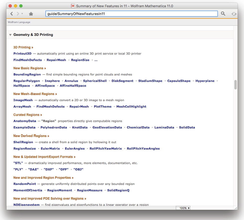
We see that there are two Plot3D options, ThickSurface and FilledSurface that will be able to generate STL files. Both approaches are illustrated as follows and illustrated in Fig. 1.4.

![]()
![]()
![]()
![]()
![]()
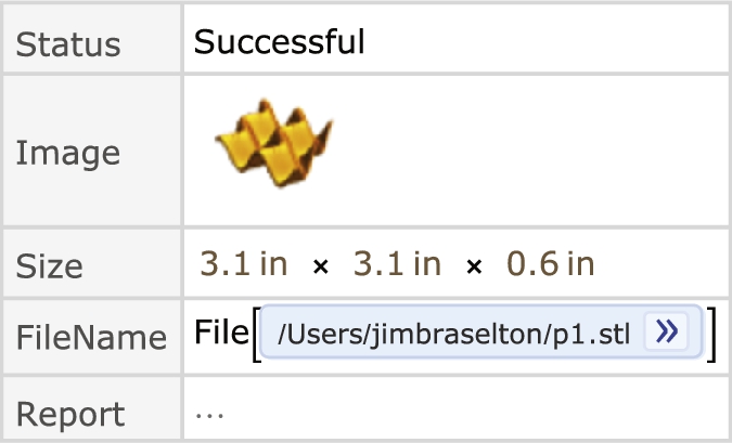
We can now save the results as an STL file, print the result to our 3D printer, or print to a 3D printing service.
Entering
![]()
saves p1 to an STL file.
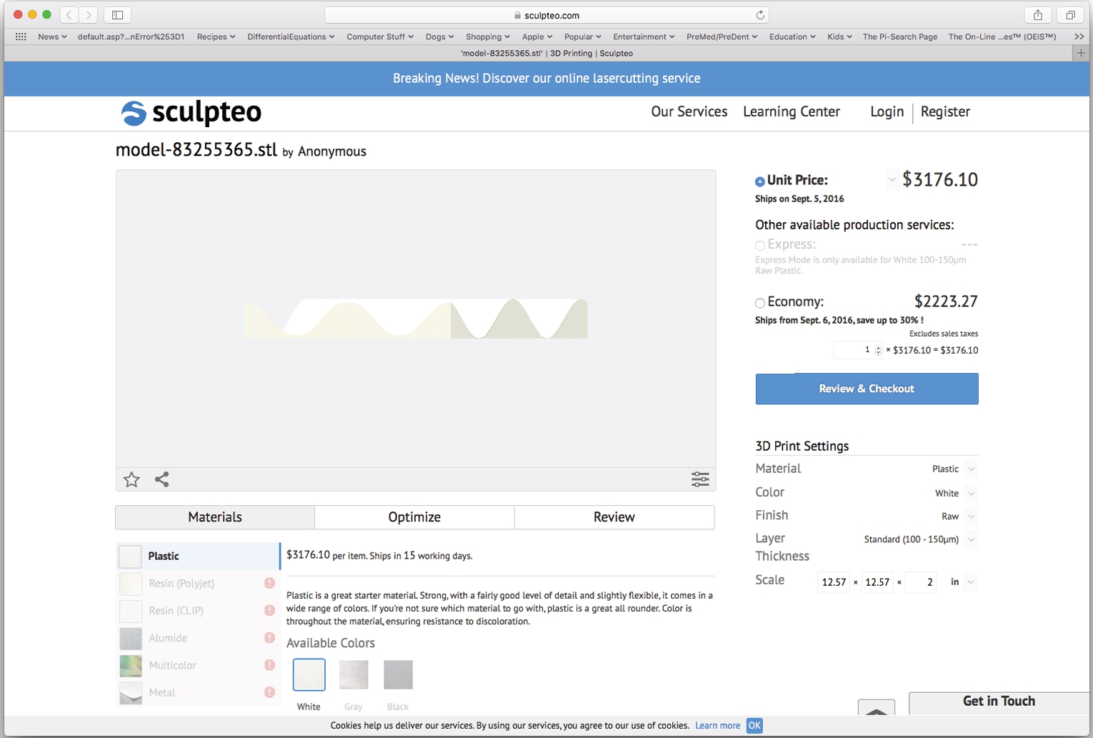
On the other hand, the following command sends the result directly to Sculpteo.
![]()
Your browser window will open and you can adjust the image to your satisfaction before ordering (or not). Many printing services are supported. You can also use this command to print directly to your own 3D printer.
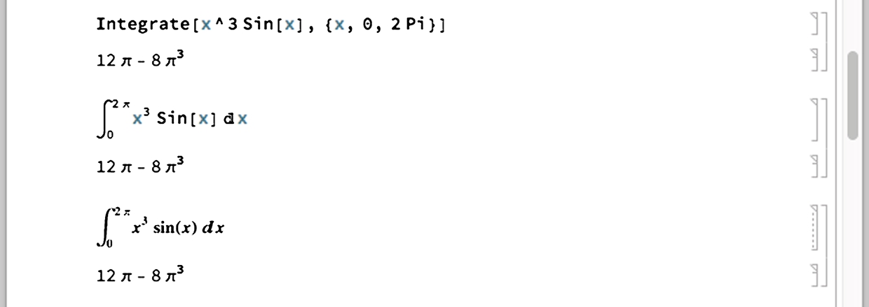
Notice that all three of the following commands
To type ![]() in Mathematica, press the
in Mathematica, press the ![]() on the Basic Math Input palette, type x in the base position, and then click (or tab to) the exponent position and type 3. Use the esc key, tab button, or mouse to help you place or remove the cursor from its current location.
on the Basic Math Input palette, type x in the base position, and then click (or tab to) the exponent position and type 3. Use the esc key, tab button, or mouse to help you place or remove the cursor from its current location.

solve the equation ![]() for x.
for x.
In the first case, the input and output are in StandardForm, in the second case the input and output are in InputForm, and in the third case, the input and output are in TraditionalForm.
To convert cells from one type to another, first select the cell, and then move the cursor to the Mathematica menu,
![]()
select Cell, and then Convert To, as illustrated in the following screen shot.

You can change how input and output appear by using ConvertTo or by changing the default settings. Moreover, you can determine the form of input/output by looking at the cell bracket that contains the input/output. For example, even though all three of the following commands look different, all three evaluate ![]() .
.
In the first calculation, the input is in Input Form and the output in Output Form, in the second the input and output are in Standard Form, and in the third the input and output are in TraditionalForm. Throughout Mathematica By Example, fifth edition, we display input and output using Input Form (for input) or Standard Form (for output), unless otherwise stated.
To enter code in Standard Form, we often take advantage of the Basic Math Input palette, which is accessed by going to Palettes under the Mathematica menu and then selecting Basic Math Input.
Use the buttons to create templates and enter special characters. Alternatively, you can access a complete list of typesetting shortcuts from Mathematica help at guide/MathematicalTypesetting in the Documentation Center.

Mathematica sessions are terminated by entering Quit[] or by selecting Quit from the File menu, or by using a keyboard shortcut, like command-Q, as with other applications. They can be saved by referring to Save from the File menu.
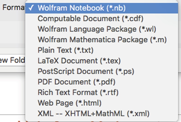
Mathematica allows you to save notebooks (as well as combinations of cells) in a variety of formats, in addition to the standard Mathematica format. From the Mathematica menu, select Save As... and then select one of the following options.
Preview
In order for the Mathematica user to take full advantage of this powerful software, an understanding of its syntax is imperative. The goal of Mathematica By Example is to introduce the reader to the Mathematica commands and sequences of commands most frequently used by beginning users of Mathematica. Although all of the rules of Mathematica syntax are far too numerous to list here, knowledge of the following five rules equips the beginner with the necessary tools to start using the Mathematica program with little trouble.
Five Basic Rules of Mathematica Syntax
1. The arguments of all functions (both built-in ones and ones that you define) are given in brackets [...]. Parentheses are (...) are used for grouping operations; vectors, matrices, and lists are given in braces {...}; and double square brackets [[...]] are used for indexing lists and tables.
2. Every word of a built-in Mathematica function begins with a capital letter.
3. Multiplication is represented by a ⁎ or space between characters. Enter 2*x*y or 2x y to evaluate ![]() not 2xy.
not 2xy.
4. Powers are denoted by a ̂. Enter (8*x^3)^(1/3) to evaluate ![]() instead of 8x^1/3, which returns 8x/3.
instead of 8x^1/3, which returns 8x/3.
5. Mathematica follows the order of operations exactly. Thus, entering (1+x)^1/x returns ![]() while (1+x)^(1/x) returns
while (1+x)^(1/x) returns ![]() . Similarly, entering x^3x returns
. Similarly, entering x^3x returns ![]() while entering x^(3x) returns
while entering x^(3x) returns ![]() .
.
6. Many calculations and tasks encountered by beginning users can be completed by filling in templates that are provided in the various palettes and accessed from the Mathematica menu. The standard Mathematica palettes are shown in Fig. 1.5.

1.2 Getting Help from Mathematica
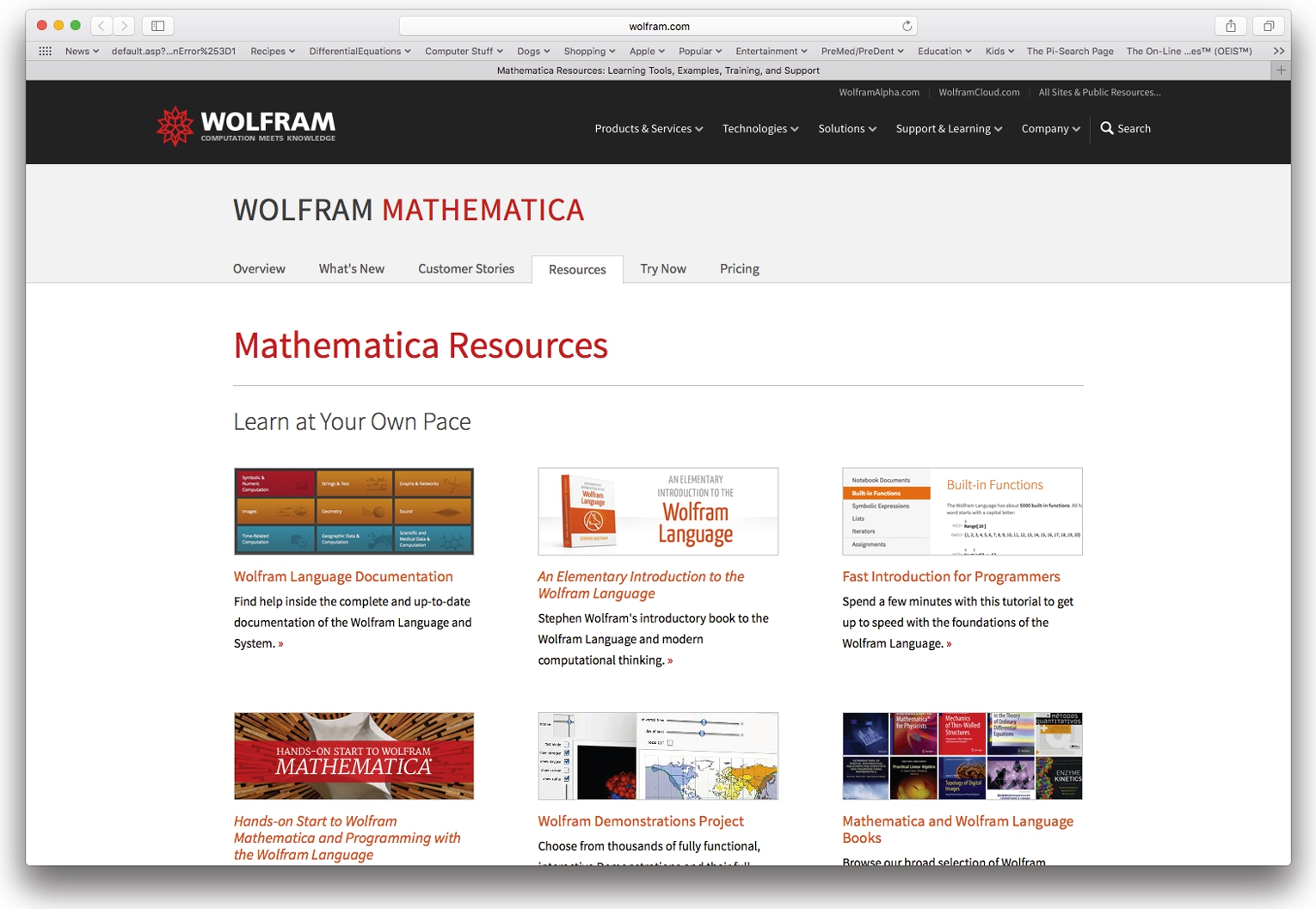
Becoming competent with Mathematica can take a serious investment of time. Hopefully, messages that result from syntax errors are viewed lightheartedly. Ideally, instead of becoming frustrated, beginning Mathematica users will find it challenging and fun to locate the source of errors. Frequently, Mathematica's error messages indicate where the error(s) has (have) occurred. In this process, it is natural that you will become more proficient with Mathematica. In addition to Mathematica's extensive help facilities, which are described next, a tremendous amount of information is available for all Mathematica users at the Wolfram Research website.
Not only can you get significant Mathematica help at the Wolfram website, you can also access outstanding mathematical resources at Wolfram's Mathematica resources that are accessed from the Welcome Screen followed by selecting Resources.
One way to obtain information about Mathematica commands and functions, including user-defined functions, is the command ?. ?object gives a basic description and syntax information of the Mathematica object object. ??object yields detailed information regarding syntax and options for the object object. Equivalently, Information[object] yields the information on the Mathematica object object returned by both ?object and Options[object] in addition to a list of attributes of object. Note that object may either be a user-defined object or a built-in Mathematica object, such as a built-in function or sequence of commands.
Solution
?Plot uses basic information about the Plot function
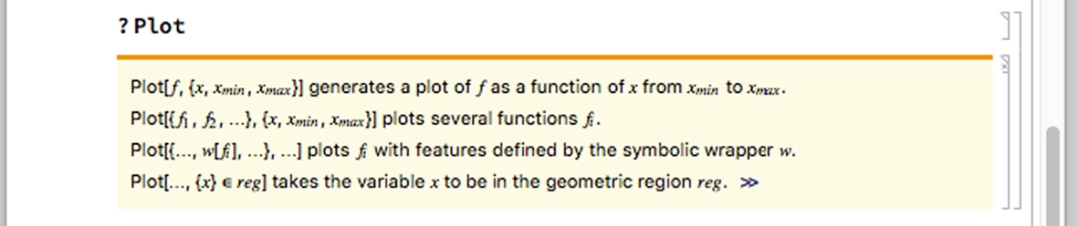
while ??Plot includes basic information as well as a list of options and their default values.
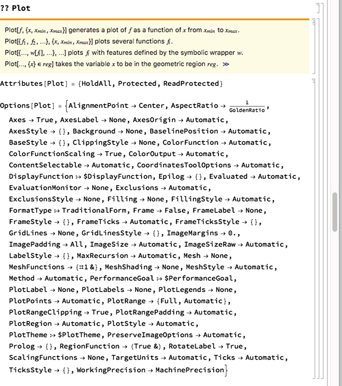
If you click on the >> button, Mathematica returns its extensive description of the function. Notice that the Plot function has been updated in Version 11. The
![]()
button shows that Plot has been updated. Click on Show Changes to see the changes in Version 11.
 □
□
Options[object] returns a list of the available options associated with object along with their current settings. This is quite useful when working with a Mathematica command such as ParametricPlot which has many options. Notice that the default value (the value automatically assumed by Mathematica ) for each option is given in the output.
Solution
The command Options[ParametricPlot] lists all the options and their current settings for the command ParametricPlot.
 □
□
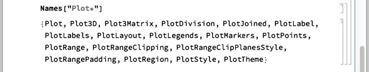
The command Names["form"] lists all objects that match the pattern defined in form. For example, Names["Plot"] returns Plot, Names["*Plot"] returns all objects that end with the string Plot, and Names["Plot*"] lists all objects that begin with the string Plot, and Names["*Plot*"] lists all objects that contain the string Plot. Names["form",SpellingCorrection->True] finds those symbols that match the pattern defined in form after a spelling correction.
Solution
We use Names to find all objects that match the pattern Plot.
![]()
Next, we use Names to create a list of all built-in functions beginning with the string Plot.
 □
□
In the following, after using ? to learn about the Mathematica function ColorData, we go to the Mathematica menu and select Palettes followed by Color Schemes.
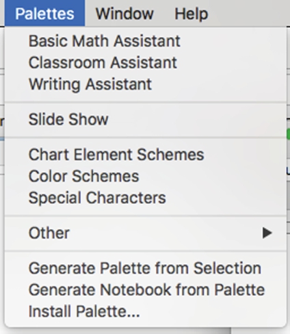
We are given a variety of choices. Using these choices is illustrated throughout Mathematica By Example.

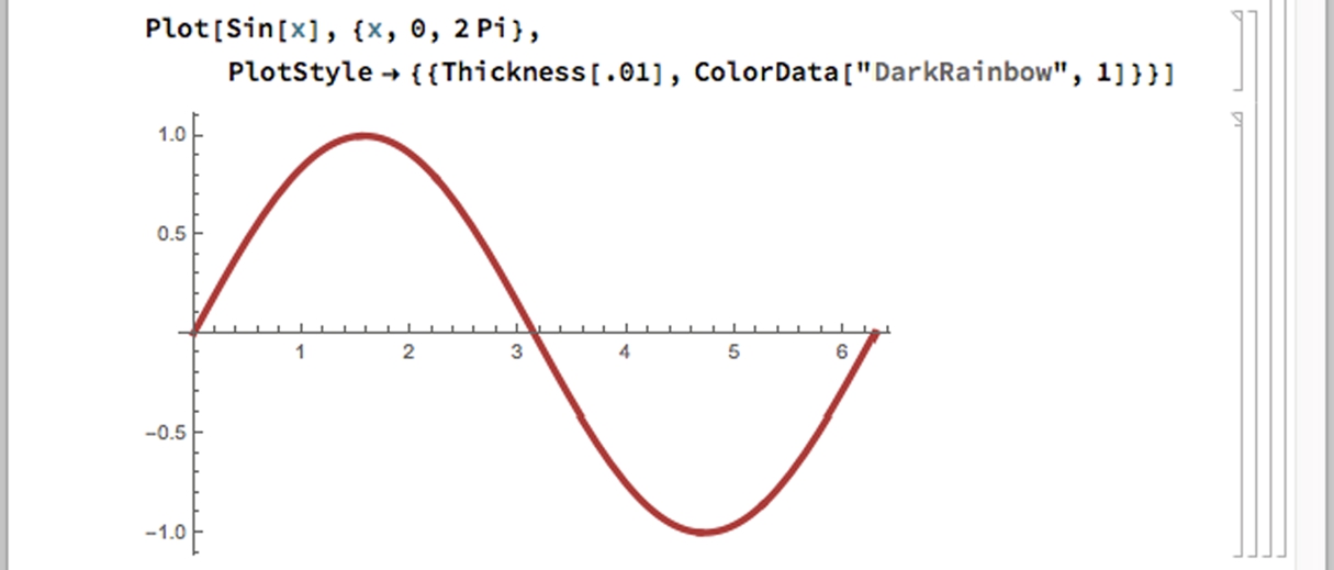
We then use the help facilities description of the ColorData function
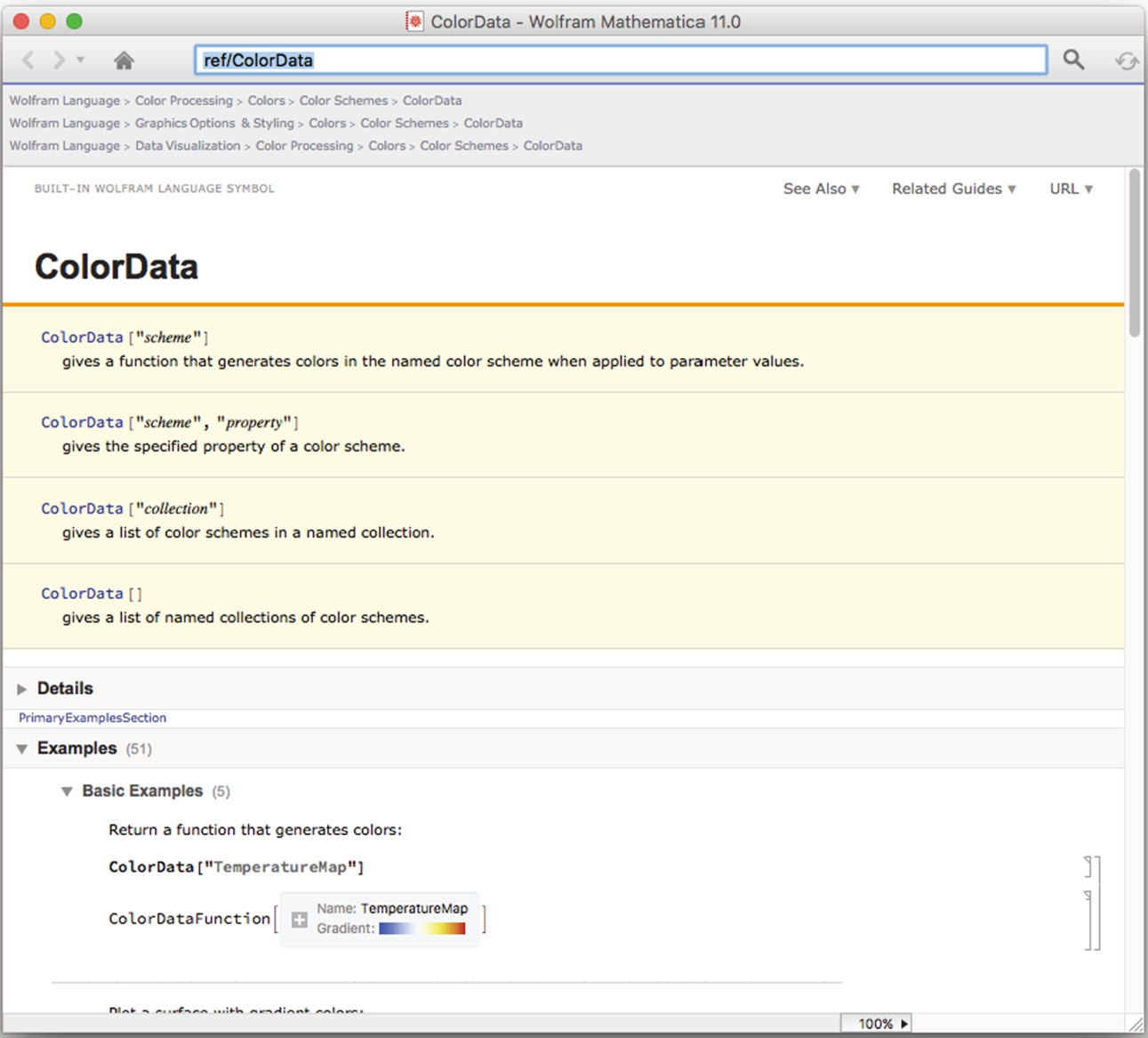
to help us generate a plot of ![]() on the interval
on the interval ![]() in deep red on our computer or that shown in the on-line version of this text.
in deep red on our computer or that shown in the on-line version of this text.
As we have illustrated, the ? function can be used in many ways. Entering ?letters* gives all Mathematica objects that begin with the string letters; ?*letters* gives all Mathematica objects that contain the string letters; and ?*letters gives all Mathematica commands that end in the string letters.
Solution
Entering

returns all functions ending with the string Cos, entering

returns all functions containing the string Sin, and entering

returns all functions that contain the string Polynomial. □
Mathematica Help
Additional help features are accessed from the Mathematica menu under Help. Although many of these topics have already been discussed, they are included again here for easy reference. For basic help information about Mathematica, go to the Mathematica menu, followed by Help and select Wolfram Documentation

From this menu, you can choose a subject and then a sub-subject. For illustrative purposes, we select Symbolic & Numeric Computation followed by Calculus.

To obtain information about a particular Mathematica object or function, open the Documentation Center, type the name of the object, function, or topic and press the Go (>) button or press Enter as we have done here with ExampleData.
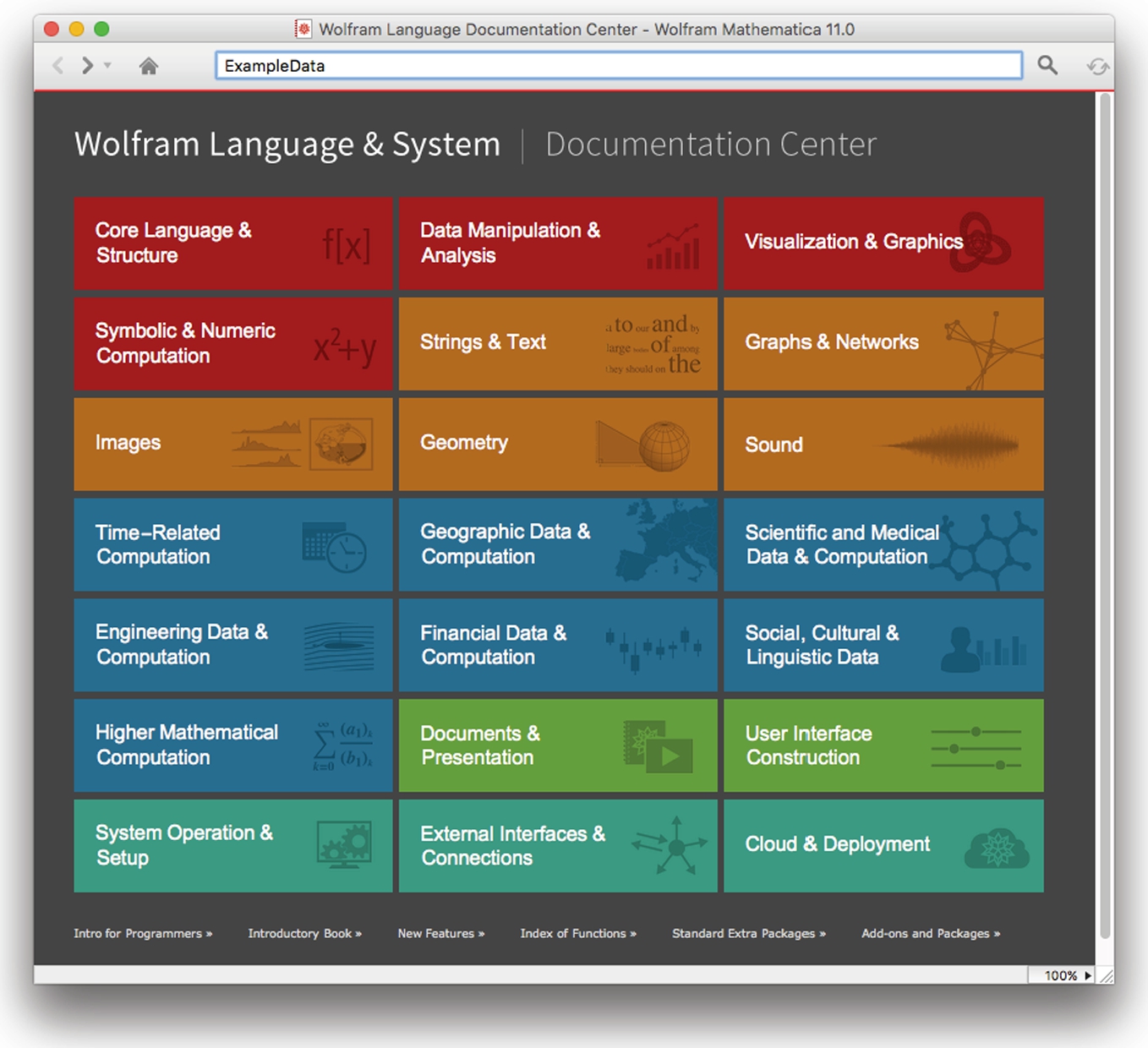
A typical help window not only contains a detailed description of the command and its options as well as hyperlinked cross-references to related commands and can be accessed by clicking on the appropriate links.

You can also use the Documentation Center to search for help regarding a particular topic. In this case we enter color schemes in the top line of the Documentation Center and then click on the > button (or press Enter) to see all the on-line help regarding “color schemes.”

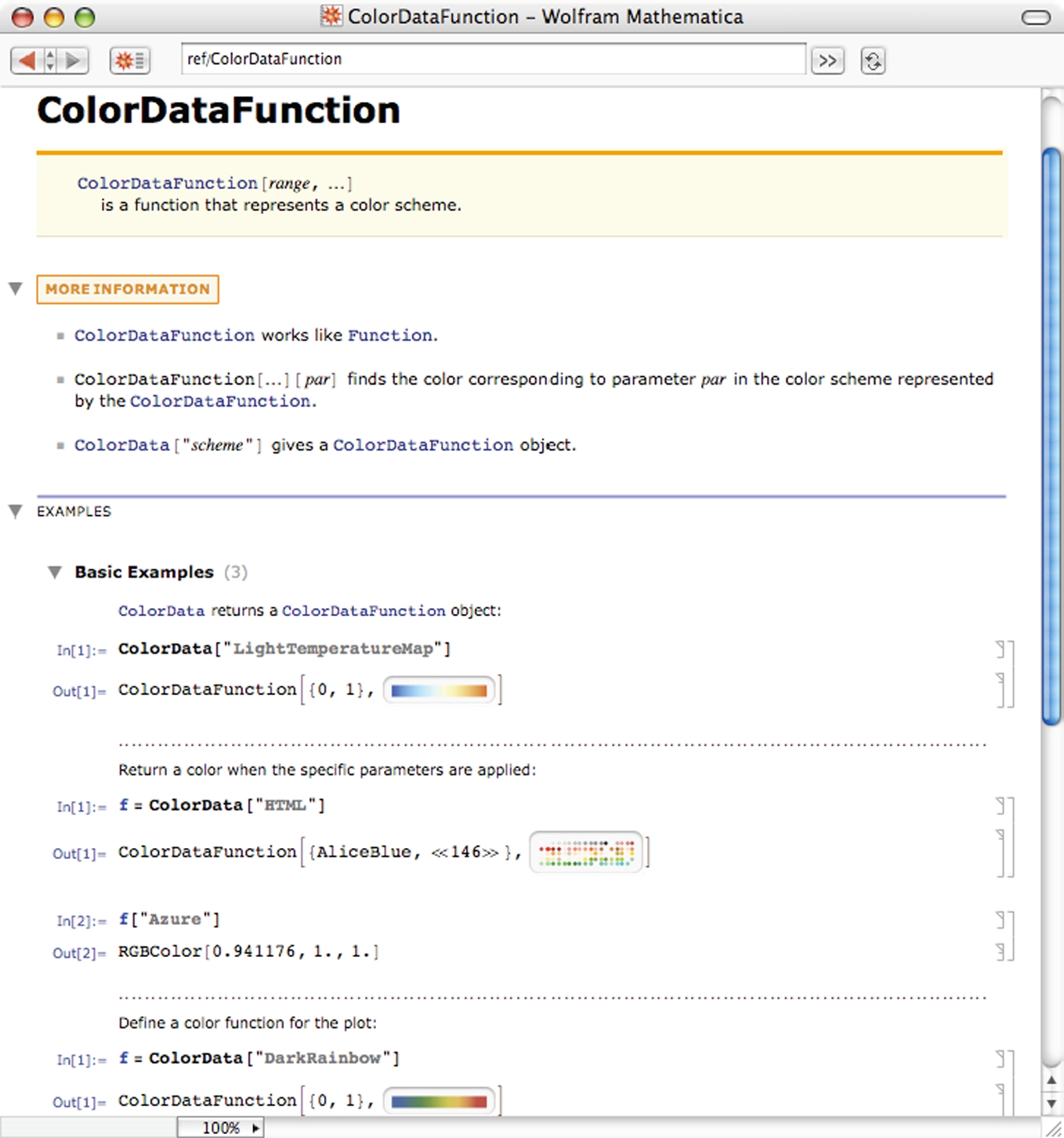
Clicking on the topic will take you to the documentation for the topic. Here is what we see when we select Color Data.
As you become more proficient with Mathematica, you will want to learn to take advantage of its extensive capabilities. Remember that Mathematica contains thousands of functions to perform many tasks. If you wish to perform a task that is not discussed here, go to the Documentation Center and type a few words related to what you want to do. For example, to investigate integer operations, we search for them.
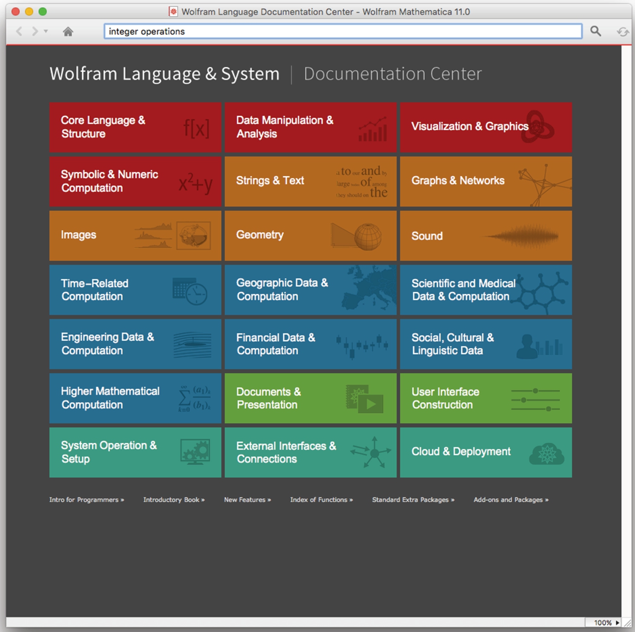
Here is the result of the search.
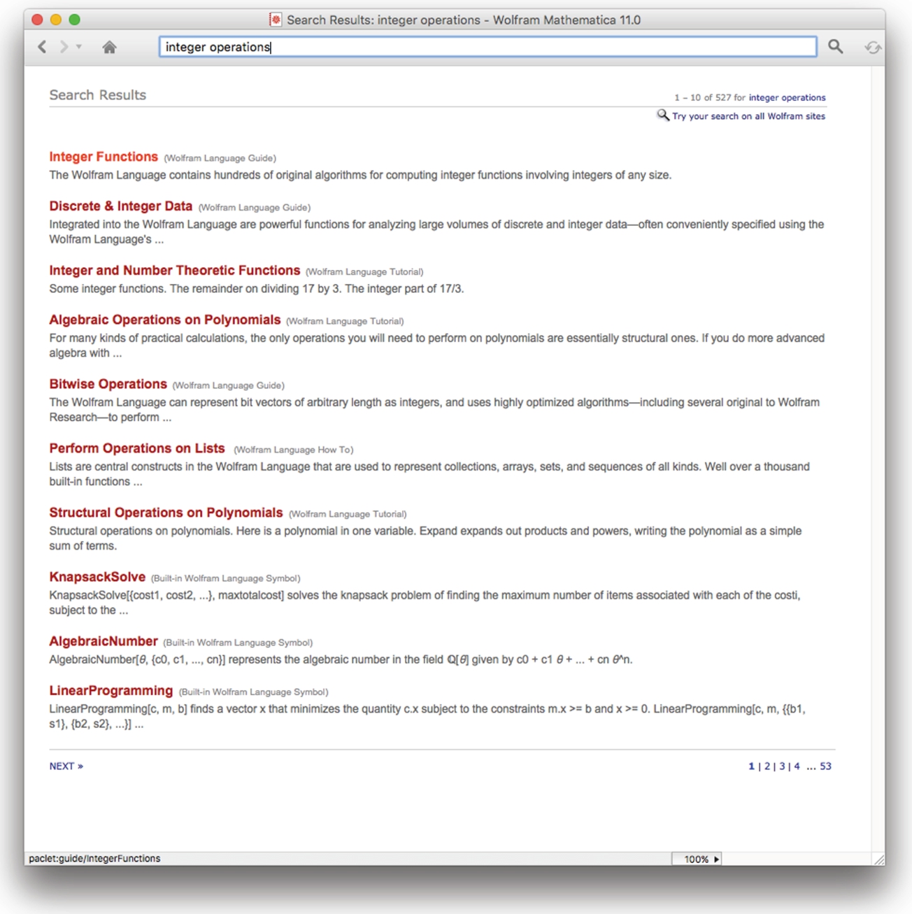
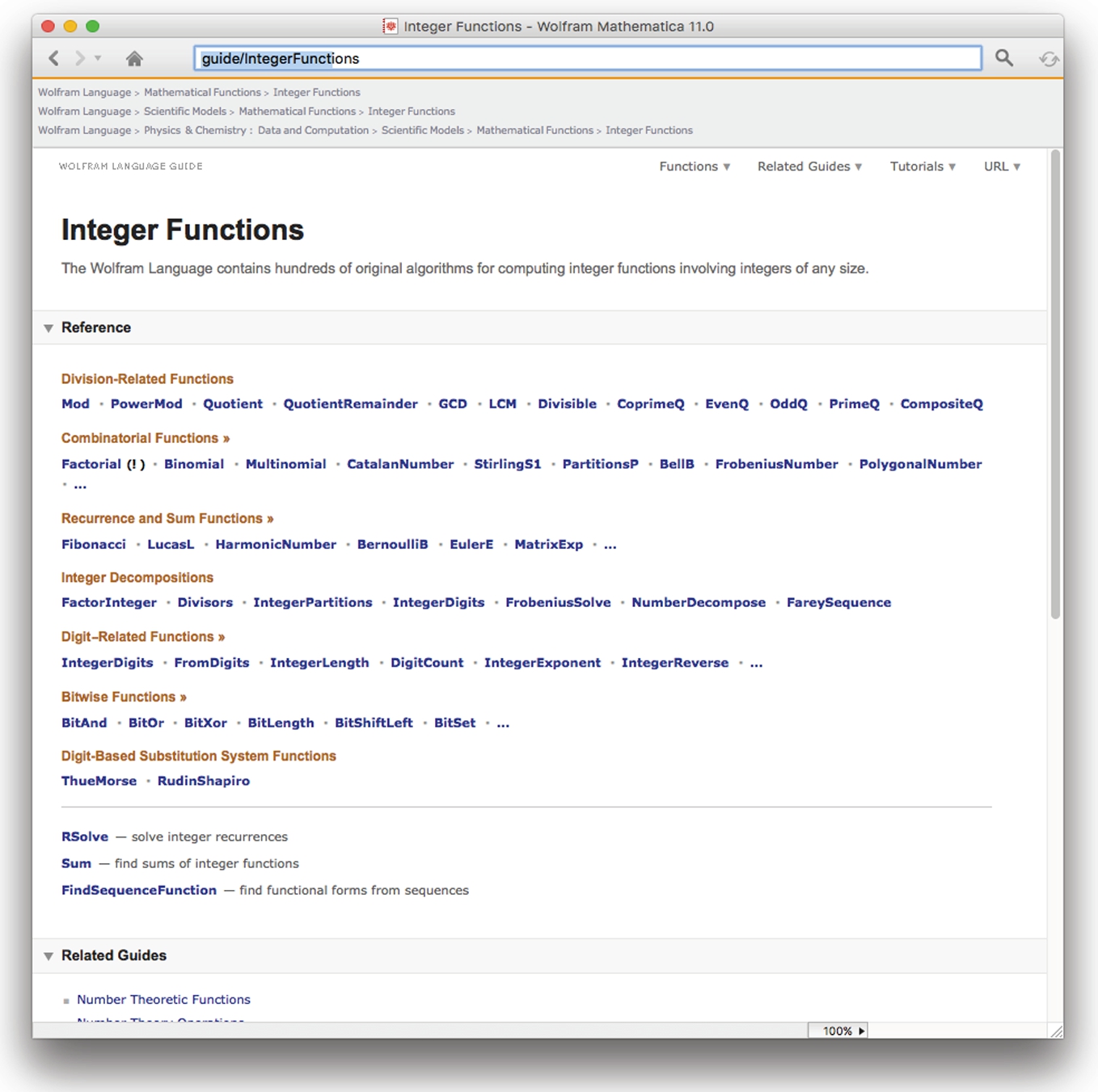
We select “Integer Functions.”
Example 1.5
In this example, we investigate digit operations. Mathematica By Example, Fifth Edition, is copyright in 2017, which has four digits.
![]()
![]()
As a string, the number is
![]()
2017
In base 2, the copyright year is
![]()
11111100001
On the other hand, with Roman numerals the copyright year for the Fourth edition is
![]()
MMVIII