Introduction to Lists and Tables
Keywords
Dynamical systems; Engineering applications; Lists; Graphing lists
4.1 Lists and List Operations
4.1.1 Defining Lists
A list of n elements is a Mathematica object of the form
list={a1,a2,a3,...,an}.
The ith element of the list is extracted from list with list[[i]] or Part[list,i].
Elements of a list are separated by commas. Lists are always enclosed in braces {...} and each element of a list may be (almost any) Mathematica object, even other lists. Because lists are Mathematica objects, they can be named. For easy reference, we will usually name lists.
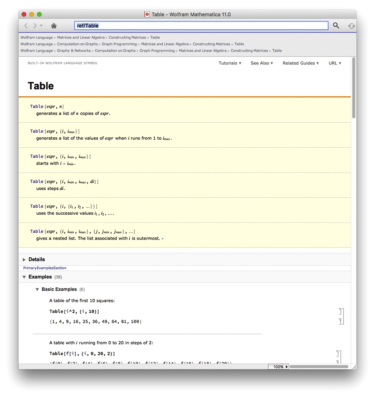
Lists can be defined in a variety of ways: they may be completely typed in, imported from other programs and text files, or they may be created with either the Table or Array commands. Given a function ![]() and a number n, the command
and a number n, the command
1. Table[f[i],{i,n}] creates the list {f[1],...,f[n]};
2. Table[f[i],{i,0,n}] creates the list {f[0],...,f[n]};
3. Table[f[i],{i,n,m}] creates the list
{f[n],f[n+1],...,f[m-1],f[m]};
4. Table[f[i],{i,imin,imax,istep}] creates the list
{f[imin],f[imin+istep],f[imin+2*istep],...,f[imax]};
and
5. Array[f,n] creates the list {f[1],...,f[n]}.
In particular,
Table[f[x],{x,a,b,(b-a)/(n-1)}]
returns a list of ![]() values for n equally spaced values of x between a and b;
values for n equally spaced values of x between a and b;
Table[{x,f[x]},{x,a,b,(b-a)/(n-1)}]
returns a list of points ![]() for n equally spaced values of x between a and b.
for n equally spaced values of x between a and b.
In addition to using Table, lists of numbers can be calculated using Range.
1. Range[n] generates the list {1,2, ... , n};
2. Range[n1,n2] generates the list {n1, n1+1, ... , n2-1, n2}; and
3. Range[n1,n2,nstep] generates the list
{n1, n1+nstep,n1+2*nstep, ... , n2-nstep,n2}.
Solution
Generally, a given list can be constructed in several ways. In fact, each of the following five commands generates the list {1,2,3,4,5,6,7,8,9,10}.
![]()
![]()
![]()
![]()
![]()
![]()
![]()
![]()
![]()
![]() □
□
Example 4.2
Use Mathematica to define listone to be the list of numbers ![]() .
.
Solution
In this case, we generate a list and name the result listone. As in Example 4.1, we illustrate that listone can be created in several ways.
![]()
![]()
![]()
![]()
Last, we define ![]() and use Array to create the table listone.
and use Array to create the table listone.
![]()
![]()
![]() □
□
Solution
The command Prime[n] yields the nth prime number. We use Table to generate a list of the ordered pairs {n,Prime[n]} for ![]() , 2, 3, …, 25 and name the resulting list list. We then use verb+Short+ to obtain an abbreviated portion of list. Generally, Short returns the first and last few elements of a list. The number of omitted terms between the first few and last few is indicated with <<n>>. In this case, we see that 13 terms are omitted.
, 2, 3, …, 25 and name the resulting list list. We then use verb+Short+ to obtain an abbreviated portion of list. Generally, Short returns the first and last few elements of a list. The number of omitted terms between the first few and last few is indicated with <<n>>. In this case, we see that 13 terms are omitted.
![]()
![]()
![]()
The ith element of a list list is extracted from list with list[[i]] or Part[list,i]. From the resulting output, we see that the fifteenth prime number is 47.
![]()
![]()
![]()
![]() □
□
In addition, we can use Table to generate lists consisting of the same or similar objects.
Solution
Entering
![]()
![]()
![]()
generates a list consisting of five copies of the letter a. For (b), we use the command RandomInteger and RandomReal to generate the desired lists. Because we are using RandomInteger and RandomReal, your results will certainly differ from those obtained here.
![]()
![]()
![]()
![]() □
□
Manipulate works in much the same way as Table but allows you to interactively see how adjusting parameters affects a given situation.
Example 4.5
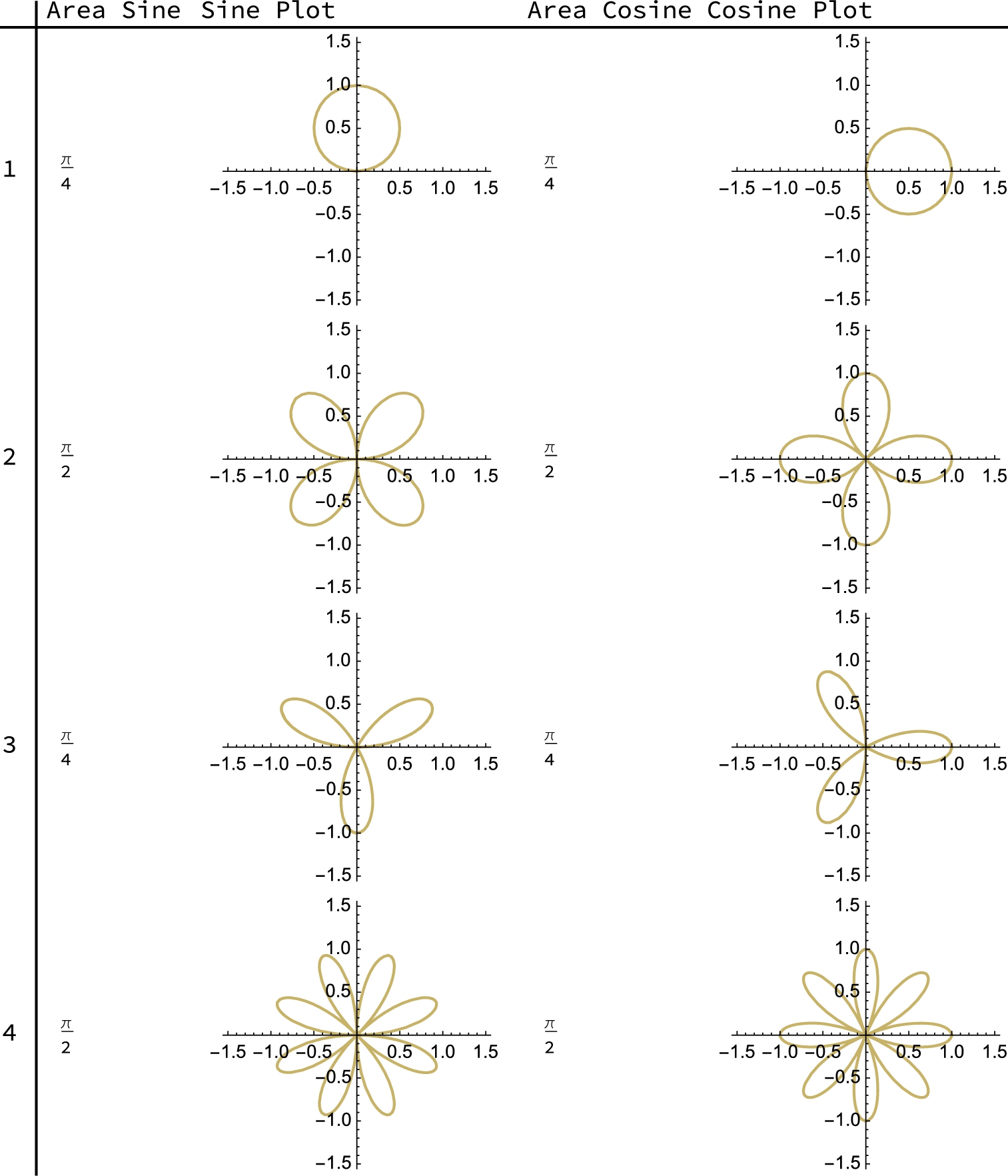
For example, in polar coordinates, the graphs of ![]() and
and ![]() are n-leaved roses if n is odd and 2n-leaved roses if n is even. If n is even, the area of the graph enclosed by the 2n roses is
are n-leaved roses if n is odd and 2n-leaved roses if n is even. If n is even, the area of the graph enclosed by the 2n roses is ![]() . While if n is odd, the area of the graph enclosed by the n roses is
. While if n is odd, the area of the graph enclosed by the n roses is ![]() .
.
To see this with Mathematica, we can use Table. (See Figs. 4.1 and 4.2.) (Note that If[condition,f,g] returns f if condition is True and g if it is not.)
![]()
![]()
![]()
![]()
![]()
![]()
![]()
![]()
![]()
![]()
![]()
![]()
![]()
![]()
![]()
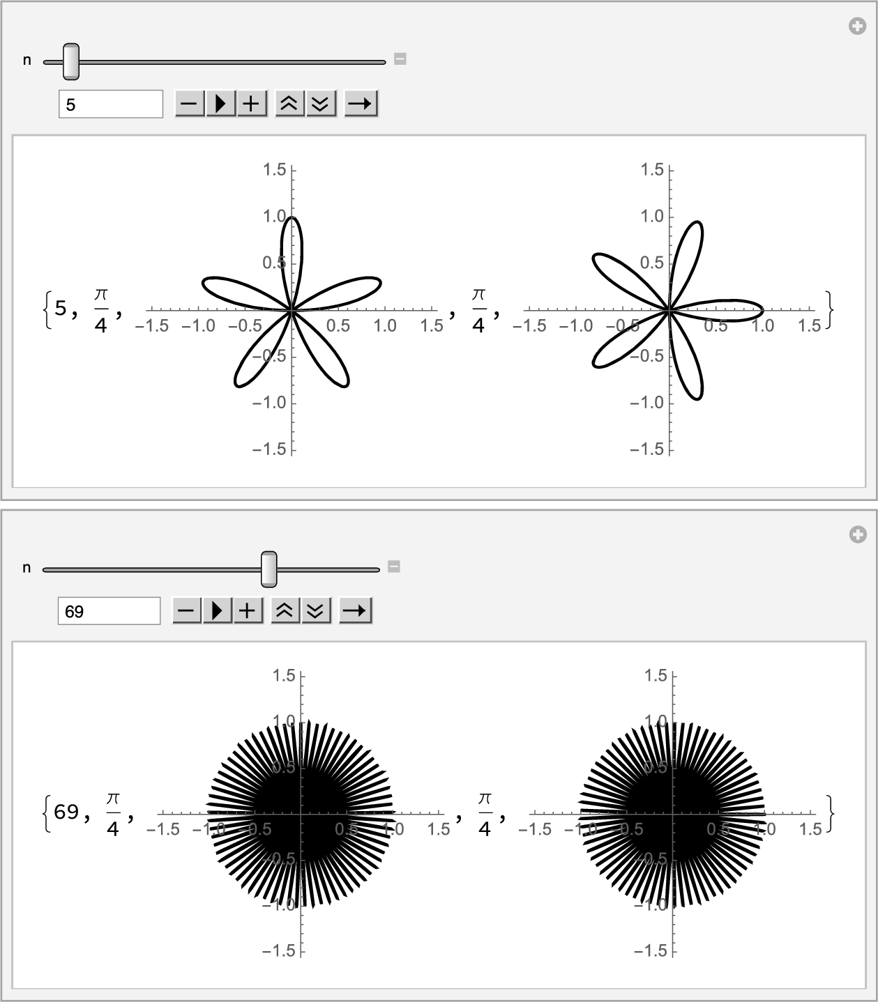
Alternatively, you can use Manipulate.
![]()
![]()
![]()
![]()
![]()
![]()
![]()
![]()
![]()
![]()
![]()
![]()
4.1.2 Plotting Lists of Points
Lists are plotted with ListPlot.
1. ListPlot[{{x1,y1},{x2,y2},...,{xn,yn}}] plots the list of points ![]() . The size of the points in the resulting plot is controlled with the option PlotStyle->PointSize[w], where w is the fraction of the total width of the graphic. For two-dimensional graphics, the default value is 0.008.
. The size of the points in the resulting plot is controlled with the option PlotStyle->PointSize[w], where w is the fraction of the total width of the graphic. For two-dimensional graphics, the default value is 0.008.
2. ListPlot[{y1,y2,..,yn}] plots the list of points ![]()
![]() .
.
3. ListLinePlot[{y1,y2,..,yn}] plots the list of points ![]()
![]() and connects consecutive points with line segments. Alternatively, you can use ListPlot together with the option Joined->True to connect consecutive points with line segments.
and connects consecutive points with line segments. Alternatively, you can use ListPlot together with the option Joined->True to connect consecutive points with line segments.
Example 4.6
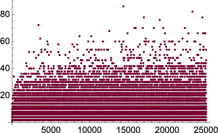
Entering
![]()
![]()
creates a list consisting of ![]() for
for ![]() , 2, …, 1000 and then graphs the list of points
, 2, …, 1000 and then graphs the list of points ![]() for
for ![]() , 2, …, 1000. See Fig. 4.3.
, 2, …, 1000. See Fig. 4.3.
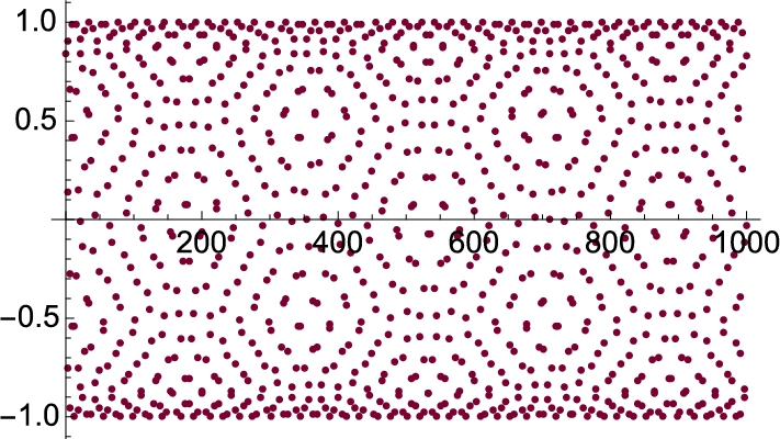
 for n = 1, 2, …, 1000. (University of Massachusetts at Amherst colors)
Example 4.7
The Prime Difference Function and the Prime Number Theorem
In t1, we use Prime and Table to compute a list of the first ![]() prime numbers.
prime numbers.
![]()
![]()
We use Length to verify that t1 has ![]() elements and Short to see an abbreviated portion of t1.
elements and Short to see an abbreviated portion of t1.
25000
![]()
![]()
You can also use Take to extract elements of lists.
1. Take[list,n] returns the first n elements of list;
2. Take[list,-n] returns the last n elements of list; and
3. Take[list,{n,m}] returns the nth through mth elements of list.
![]()
![]()
![]()
![]()
![]()
![]()
In t2, we compute the difference, ![]() , between the successive prime numbers in t1. The result is plotted with ListPlot in Fig. 4.4.
, between the successive prime numbers in t1. The result is plotted with ListPlot in Fig. 4.4.
list[[i]] returns the ith element of list so ![]() computes the difference between the
computes the difference between the ![]() st and ith elements of list. list[[i,j]] returns the jth part of the ith part of list.
st and ith elements of list. list[[i,j]] returns the jth part of the ith part of list.
![]()
![]()
![]()
![]()
![]()
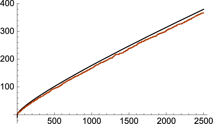
Let ![]() denote the number of primes less than n and
denote the number of primes less than n and ![]() denote the logarithmic integral:
denote the logarithmic integral:
We use Plot to graph ![]() for
for ![]() in p1.
in p1.
![]()
![]()
The Prime Number Theorem states that
(See [17].) In the following, we use Select and Length to define ![]() . Select[list,criteria] returns the elements of list for which criteria is true. Note that #<n is called a pure function: given an argument #, #<n is true if #<n and false otherwise. The & symbol marks the end of a pure function. Thus, given n, Select[t1,#<n&] returns a list of the elements of t1 less than n; Select[t1,#<n&]//Length returns the number of elements in the list.
. Select[list,criteria] returns the elements of list for which criteria is true. Note that #<n is called a pure function: given an argument #, #<n is true if #<n and false otherwise. The & symbol marks the end of a pure function. Thus, given n, Select[t1,#<n&] returns a list of the elements of t1 less than n; Select[t1,#<n&]//Length returns the number of elements in the list.
![]()
For example,
![]()
25
shows us that ![]() . Note that because t1 contains the first
. Note that because t1 contains the first ![]() primes, smallpi[n] is valid for
primes, smallpi[n] is valid for ![]() where
where ![]() . In t3, we compute
. In t3, we compute ![]() for
for ![]() , 2, …, 2500
, 2, …, 2500
![]()
![]()
![]()
and plot the resulting list with ListPlot.
![]()
p1 and p2 are displayed together with Show in Fig. 4.5.
![]()
Working in almost the same way as Take, Span (;;) selects elements of lists: list[[n;;m]] returns the n through mth elements of list.
Example 4.8
Here are the first few terms of sequence A073184 (N.J.A. Sloane, 2007, The On-Line Encyclopedia of Integer Sequences, www.research.att.com/njas/sequences/), the number of cube free divisors of n.
![]()
![]()
![]()
With ;; (Span), we select the 2nd through 8th elements of ashortlist.
![]()
![]()
The same results are obtained with Take.
![]()
![]()
You can count the number of elements of a list with Length.
![]()
35
With Tally, we count the number of occurrences of each digit in the list. Thus,
![]()
![]()
shows us that there are 11 2's, 10 4's, and so on.
However, you can use Table together with Part ([[...]]) to obtain the same results as those obtained with Take or Span.
![]()
![]()
![]()
![]()
![]()
![]()
You can iterate recursively with Table. Both
![]()
![]()
![]()
![]()
5
and
![]()
![]()
compute tables of ![]() . The outermost iterator is evaluated first: in this case, i is followed by j as in t1 and the result is a list of lists. To eliminate the inner lists (that is, the braces), use Flatten. Generally, Flatten[list,n] flattens list (removes braces) to level n.
. The outermost iterator is evaluated first: in this case, i is followed by j as in t1 and the result is a list of lists. To eliminate the inner lists (that is, the braces), use Flatten. Generally, Flatten[list,n] flattens list (removes braces) to level n.
![]()
![]()
The observation is especially important when graphing lists of points obtained by iterating Table. For example,
![]()
![]()
![]()
5
is not a list of 25 points: t1 is a list of 5 lists each consisting of 5 points. t1 has two levels. For example, the 3rd element of the second level is
![]()
![]()
and the 2nd element of the third level (or the second part of the third part) is
![]()
![]()
To flatten t2 to level 1, we use Flatten.
![]()
![]()
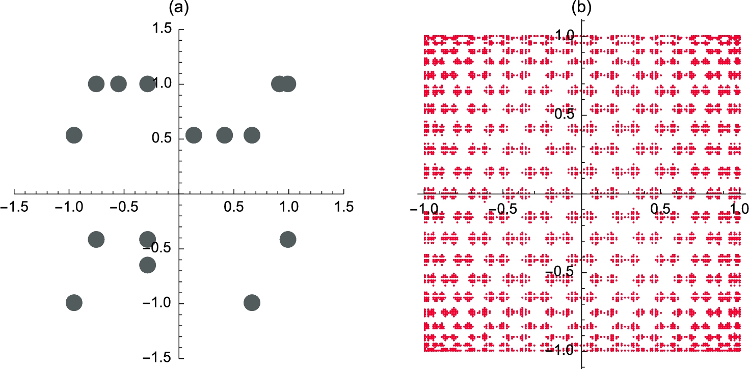
The resulting list of ordered pairs (in Mathematica, {x,y} corresponds to ![]() ). This list of points are then plotted with ListPlot in Fig. 4.6 (a). We also illustrate the use of the PlotStyle, PlotRange, and AspectRatio options in the ListPlot command.
). This list of points are then plotted with ListPlot in Fig. 4.6 (a). We also illustrate the use of the PlotStyle, PlotRange, and AspectRatio options in the ListPlot command.
![]()
![]()
![]()
Increasing the number of points further illustrates the use of Flatten. Entering
![]()
![]()
125
results in a very long nested list. t1 has 125 elements each of which has 125 elements.
An abbreviated version is viewed with Short.
![]()
![]()
After using Flatten, we see with Length and Short that t2 contains 15, 625 points,
![]()
![]()
15625
![]()
![]()
which are plotted with ListPlot in Fig. 4.6 (b).
![]()
![]()
![]()
Example 4.9
Dynamical Systems
A sequence of the form ![]() is called a dynamical system.
is called a dynamical system.
Observe that ![]() can also be computed with
can also be computed with ![]() .
.
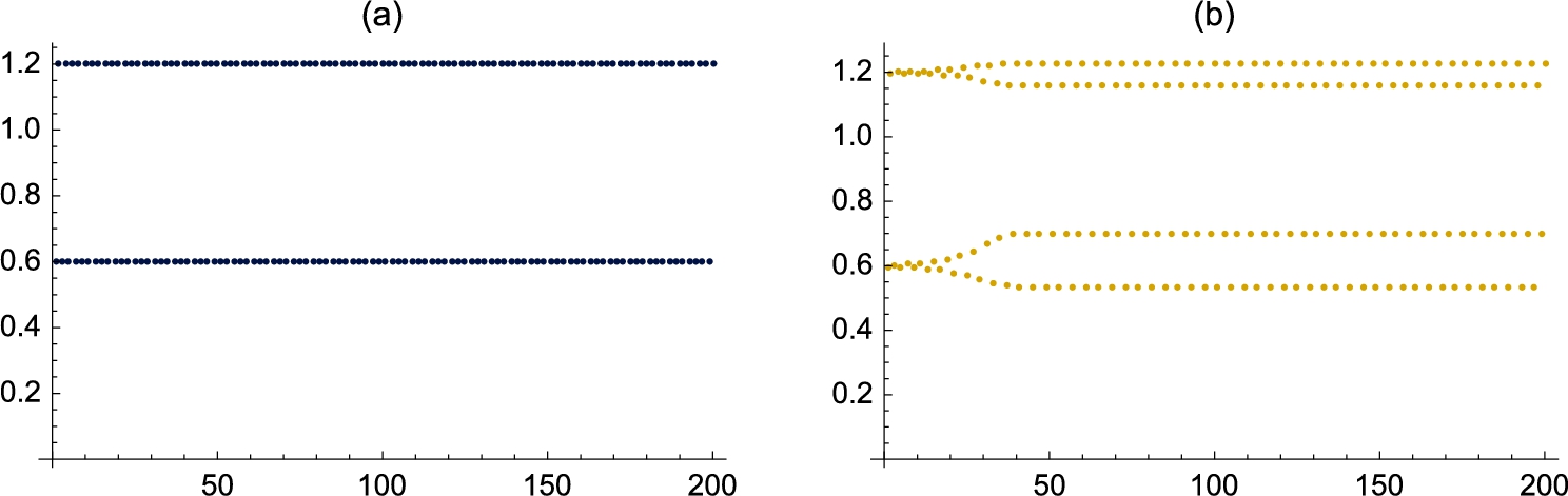
Sometimes, unusual behavior can be observed when working with dynamical systems. For example, consider the dynamical system with ![]() and
and ![]() . Note that we define
. Note that we define ![]() using the form x[n_]:=x[n]=... so that Mathematica “remembers” the functional values it computes and thus avoids recomputing functional values previously computed. This is particularly advantageous when we compute the value of
using the form x[n_]:=x[n]=... so that Mathematica “remembers” the functional values it computes and thus avoids recomputing functional values previously computed. This is particularly advantageous when we compute the value of ![]() for large values of n.
for large values of n.
![]()
![]()
![]()
![]()
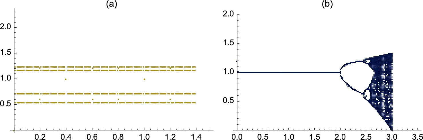
In Fig. 4.7 (a), we see that the sequence ![]() oscillates between the numbers 0.6 and 1.2. We say that the dynamical system has a 2-cycle because the values of the sequence oscillate between two numbers.
oscillates between the numbers 0.6 and 1.2. We say that the dynamical system has a 2-cycle because the values of the sequence oscillate between two numbers.
![]()
![]()
![]()
In Fig. 4.7 (b), we see that changing ![]() from 1.2 to 1.201 results in a 4-cycle.
from 1.2 to 1.201 results in a 4-cycle.
![]()
![]()
![]()
![]()
![]()
![]()
![]()
![]()
The calculations indicate that the behavior of the system can change considerably for small changes in ![]() . With the following, we adjust the definition of x so that x depends on
. With the following, we adjust the definition of x so that x depends on ![]() : given c,
: given c, ![]() .
.
![]()
![]()
![]()
![]()
In tb, we create a list of lists of the form ![]() for 150 equally spaced values of c between 0 and 1.5. Observe that Mathematica issues several error messages. When a Mathematica calculation is larger than the machine's precision, we obtain an Overflow warning. In numerical calculations, we interpret Overflow to correspond to ∞.
for 150 equally spaced values of c between 0 and 1.5. Observe that Mathematica issues several error messages. When a Mathematica calculation is larger than the machine's precision, we obtain an Overflow warning. In numerical calculations, we interpret Overflow to correspond to ∞.
![]()
![]()
![]()
![]()
![]()
We ignore the error messages and use Short to view an abbreviated form of tb.
![]()
![]()
We then use Flatten to convert tb to a list of points which are plotted with ListPlot in Fig. 4.8 (a).
![]()
![]()
![]()
Another interesting situation occurs if we fix ![]() and let c vary in
and let c vary in ![]() .
.
With the following we set ![]() and adjust the definition of f so that f depends on c:
and adjust the definition of f so that f depends on c: ![]() .
.
![]()
![]()
![]()
![]()
In tb, we create a list of lists of the form ![]() for 350 equally spaced values of c between 0 and 3.5. As before, Mathematica issues several error messages, which we ignore.
for 350 equally spaced values of c between 0 and 3.5. As before, Mathematica issues several error messages, which we ignore.
![]()
![]()
![]()
![]()
![]()
![]()
![]()
tb is then converted to a list of points with Flatten and the resulting list is plotted in Fig. 4.8 (b) with ListPlot. This plot is called a bifurcation diagram.
![]()
![]()
![]()
![]()
As indicated earlier, elements of lists can be numbers, ordered pairs, functions, and even other lists. You can also use Mathematica to manipulate lists in numerous ways. Most importantly, the Map function is used to apply a function to a list: Map[f,{x1,x2,...,xn}] returns the list ![]() . We will discuss other operations that can be performed on lists in the following sections.
. We will discuss other operations that can be performed on lists in the following sections.
Example 4.10
Hermite Polynomials
The Hermite polynomials, ![]() , satisfy the differential equation
, satisfy the differential equation ![]() and the orthogonality relation
and the orthogonality relation
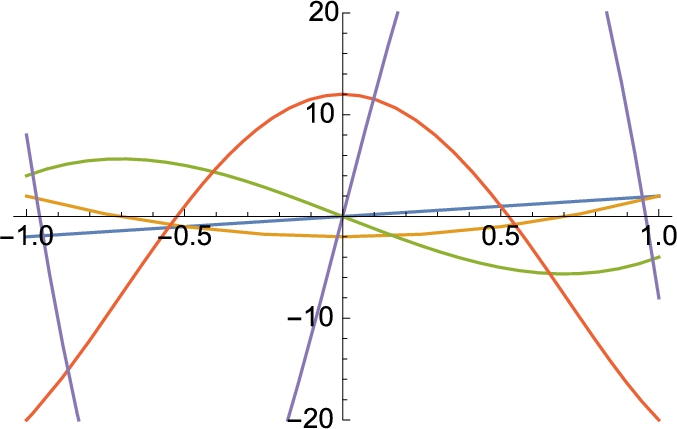
The Mathematica command HermiteH[n,x] yields the Hermite polynomial ![]() . (a) Create a table of the first five Hermite polynomials. (b) Evaluate each Hermite polynomial if
. (a) Create a table of the first five Hermite polynomials. (b) Evaluate each Hermite polynomial if ![]() . (c) Compute the derivative of each Hermite polynomial in the table. (d) Compute an antiderivative of each Hermite polynomial in the table. (e) Graph the five Hermite polynomials on the interval
. (c) Compute the derivative of each Hermite polynomial in the table. (d) Compute an antiderivative of each Hermite polynomial in the table. (e) Graph the five Hermite polynomials on the interval ![]() . (f) Verify that
. (f) Verify that ![]() satisfies
satisfies ![]() for
for ![]() (′ denotes
(′ denotes ![]() ).
).
Solution
We proceed by using HermiteH together with Table to define hermitetable to be the list consisting of the first five Hermite polynomials.
![]()
![]()
We then use ReplaceAll (->) to evaluate each member of hermitetable if x is replaced by 1.
![]()
![]()
Functions like D and Integrate are listable. A function is listable if it automatically passes through a list. For example, since D is listable, the command D[listoffunctions,x] will return a list of the derivative of the list listoffunctions with respect to x. Thus, each of the following commands differentiate each element of hermitetable with respect to x. In the second case, we have used a pure function: given an argument #, D[#,x]& differentiates # with respect to x. Use the & symbol to indicate the end of a pure function.
![]()
![]()
![]()
![]()
Similarly, we use Integrate to antidifferentiate each member of hermitetable with respect to x. Remember that Mathematica does not automatically include the “+C” that we include when we antidifferentiate.
![]()
![]()
![]()
![]()
To graph the list hermitetable, we use Plot to plot each function in the set hermitetable on the interval ![]() in Fig. 4.9. In this case, we specify that the displayed y-values correspond to the interval [−20, 20]. Because we apply Tooltip to the set of functions being plotted, you can identify each curve by moving the cursor and placing it over each curve to see which function is being plotted.
in Fig. 4.9. In this case, we specify that the displayed y-values correspond to the interval [−20, 20]. Because we apply Tooltip to the set of functions being plotted, you can identify each curve by moving the cursor and placing it over each curve to see which function is being plotted.
![]()
hermitetable[[n]] returns the nth element of hermitetable, which corresponds to ![]() . Thus,
. Thus,
![]()
![]()
![]()
computes and simplifies ![]() for
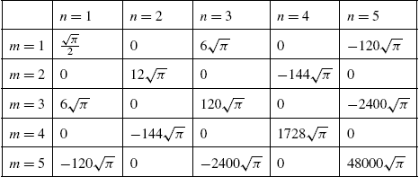
for ![]() , 2, …, 5. We use Table and Integrate to compute
, 2, …, 5. We use Table and Integrate to compute ![]() for
for ![]() , 2, …, 5 and
, 2, …, 5 and ![]() ,
, ![]() .
.
![]()
![]()
![]()
To view a table in traditional row-and-column form use TableForm, as we do here illustrating the use of the TableHeadings option.
![]()
![]()
![]()
Be careful when using TableForm: TableForm[table] is no longer a list and cannot be manipulated like a list. □
4.2 Manipulating Lists: More on Part and Map
Often, Mathematica's output is given to us as a list that we need to use in subsequent calculations. Elements of a list are extracted with Part ([[...]]): list[[i]] returns the ith element of list; list[[i,j]] (or list[[i]][[j]]) returns the jth element of the ith element of list, and so on.
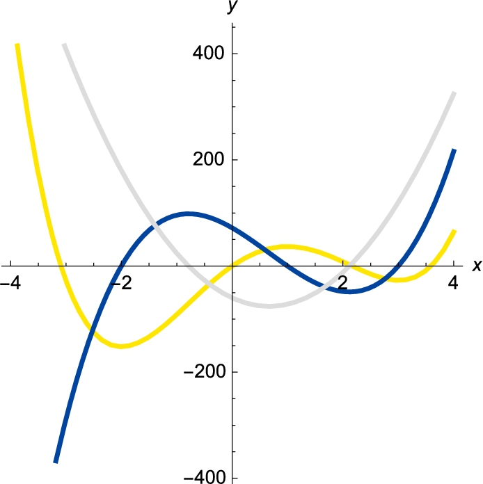
Example 4.11
Let ![]() . Locate and classify the critical points of
. Locate and classify the critical points of ![]() .
.
Solution
We begin by clearing all prior definitions of f and then defining ![]() . The critical numbers are found by solving the equation
. The critical numbers are found by solving the equation ![]() . The resulting list is named critnums.
. The resulting list is named critnums.
![]()
![]()
![]()
![]()
critnums is actually a list of lists. For example, the number −2 is the second part of the first part of the second part of critnums.
![]()
![]()
![]()
![]()
![]()
−2
Similarly, the numbers 1 and 3 are extracted with critnums[[2,1,2]] and
critnums[[3,1,2]], respectively.
![]()
![]()
1
3
We locate and classify the points by evaluating ![]() and
and ![]() for each of the numbers in critnums. f[x]/.x->a replaces each occurrence of x in
for each of the numbers in critnums. f[x]/.x->a replaces each occurrence of x in ![]() by a, so entering
by a, so entering
![]()
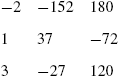
replaces each x in the list ![]() by each of the x-values in critnums.
by each of the x-values in critnums.
By the Second Derivative Test, we conclude that ![]() has relative minima at the points
has relative minima at the points ![]() and
and ![]() while
while ![]() has a relative maximum at
has a relative maximum at ![]() . In fact, because
. In fact, because ![]() , −152 is the absolute minimum value of
, −152 is the absolute minimum value of ![]() . These results are confirmed by the graph of
. These results are confirmed by the graph of ![]() in Fig. 4.10.
in Fig. 4.10.
![]()
![]()
![]()
![]()
![]() □
□
Map is a very powerful and useful function: Map[f,list] creates a list consisting of elements obtained by evaluating f for each element of list, provided that each member of list is an element of the domain of f. Note that if f is listable, f[list] produces the same result as Map[f,list].
Example 4.12
Entering
![]()
![]()
![]()
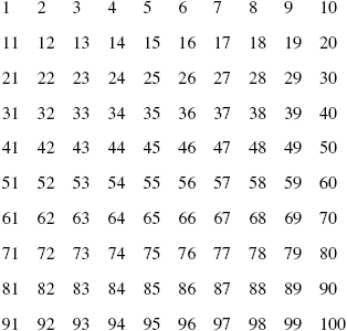
computes a list of the first 100 integers and names the result t1. To see t1, we use Partition to partition t1 in 10 element subsets; the results are displayed in a standard row-and-column form with TableForm. We then define ![]() and use Map to square each number in t1.
and use Map to square each number in t1.
![]()
![]()
![]()
![]()
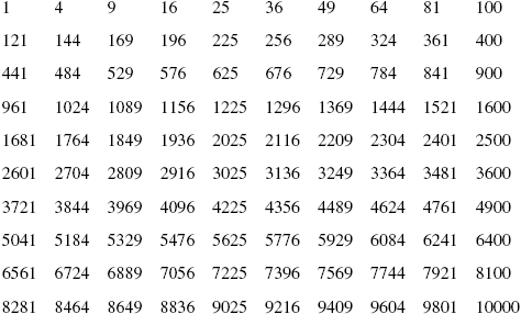
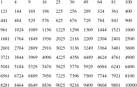
The same result is accomplished by the pure function that squares its argument. Note how # denotes the argument of the pure function; the & symbol marks the end of the pure function.
![]()
![]()
![]()
On the other hand, entering
![]()
![]()
![]()
is a list (of length 5) of lists (each of length 5). Use Flatten to obtain a list of 25 points, which we name t2.
![]()
![]()
![]()
We then use Map to apply f to t2.
![]()
![]()
![]()
![]()
We accomplish the same result with a pure function. Observe how #[[1]] and #[[2]] are used to represent the first and second arguments: given a list of length 2, the pure function returns the list of ordered pairs consisting of the first element of the list, the second element of the list (as an ordered pair), and the sum of the squares of the first and second elements (of the first ordered pair).
![]()
![]()
![]()
Example 4.13
Make a table of the values of the trigonometric functions ![]() ,
, ![]() , and
, and ![]() for the principal angles.
for the principal angles.
Solution
We first construct a list of the principal angles which is accomplished by defining t1 to be the list consisting of ![]() for
for ![]() , 1, …, 8 and t2 to be the list consisting of
, 1, …, 8 and t2 to be the list consisting of ![]() for
for ![]() , 1, …, 12. The principal angles are obtained by taking the union of t1 and t2. Union[t1,t2] joins the lists t1 and t2, removes repeated elements, and sorts the results. If we did not wish to remove repeated elements and sort the result, the command Join[t1,t2] concatenates the lists t1 and t2.
, 1, …, 12. The principal angles are obtained by taking the union of t1 and t2. Union[t1,t2] joins the lists t1 and t2, removes repeated elements, and sorts the results. If we did not wish to remove repeated elements and sort the result, the command Join[t1,t2] concatenates the lists t1 and t2.
![]()
![]()
![]()
![]()
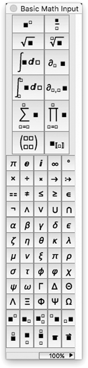
We can also use the symbol ∪, which is obtained by clicking on the ![]() button on the BasicMathInput palette to represent Union.
button on the BasicMathInput palette to represent Union.
The BasicMathInput palette:
![]()
![]()
Next, we define ![]() to be the function that returns the ordered quadruple
to be the function that returns the ordered quadruple
and compute the value of ![]() for each number in prinangles with Map naming the resulting table prinvalues. prinvalues is not displayed because a semi-colon is included at the end of the command.
for each number in prinangles with Map naming the resulting table prinvalues. prinvalues is not displayed because a semi-colon is included at the end of the command.
![]()
![]()
![]()
Finally, we use TableForm illustrating the use of the TableHeadings option to display prinvalues in row-and-column form; the columns are labeled x, ![]() ,
, ![]() , and
, and ![]() .
.
![]()
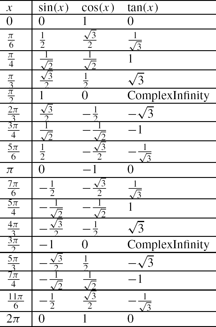
In the table, note that ![]() is undefined at odd multiples of
is undefined at odd multiples of ![]() and Mathematica appropriately returns ComplexInfinity at those values of x for which
and Mathematica appropriately returns ComplexInfinity at those values of x for which ![]() is undefined. □
is undefined. □
Lists of functions are graphed with Plot: Plot[listoffunctions,{x,a,b}] graphs the list of functions of x, listoffunctions, for ![]() . If the command is entered as Plot[Tooltip[listoffunctions],{x,a,b}], you can identify the curves in the plot by moving the cursor over the curves in the graphic.
. If the command is entered as Plot[Tooltip[listoffunctions],{x,a,b}], you can identify the curves in the plot by moving the cursor over the curves in the graphic.
Example 4.14
Bessel Functions
The Bessel functions of the first kind, ![]() , are nonsingular solutions of
, are nonsingular solutions of ![]() . BesselJ[n,x] returns
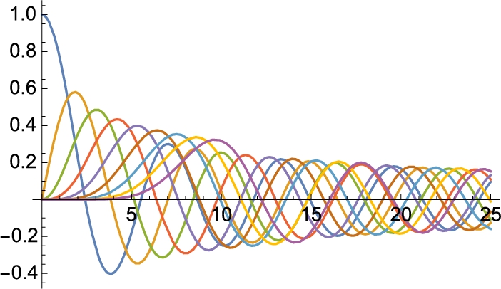
. BesselJ[n,x] returns ![]() . Graph
. Graph ![]() for
for ![]() , 1, 2, …, 8.
, 1, 2, …, 8.
Solution
In t1, we use Table and BesselJ to create a list of ![]() for
for ![]() , 1, 2, …, 8.
, 1, 2, …, 8.
![]()
We then use Plot to graph each function in t1 in Fig. 4.11. You can identify each curve by sliding the cursor over each.
![]()
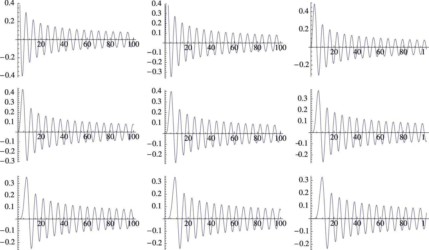
A different effect is achieved by graphing each function separately. To do so, we define the function pfunc. Given a function of x, f, pfunc[f] plots the function for ![]() . The resulting graphic is not displayed because the option DisplayFunction->Identity is included in the Plot command. We then use Map to apply pfunc to each element of t1. The result is a list of 9 graphics objects, which we name t2. A nice way to display 9 graphics is as a
. The resulting graphic is not displayed because the option DisplayFunction->Identity is included in the Plot command. We then use Map to apply pfunc to each element of t1. The result is a list of 9 graphics objects, which we name t2. A nice way to display 9 graphics is as a ![]() array so we use Partition to convert t2 from a list of length 9 to a list of lists, each with length 3 – a
array so we use Partition to convert t2 from a list of length 9 to a list of lists, each with length 3 – a ![]() array. Partition[list,n] returns a list of lists obtained by partitioning list into n-element subsets.
array. Partition[list,n] returns a list of lists obtained by partitioning list into n-element subsets.
![]()
![]()
![]()
Instead of defining pfunc, you can use a pure function instead. The following accomplishes the same result. We display t3 using Show together with GraphicsGrid in Fig. 4.12.
![]()
![]()
![]()
![]() □
□
Example 4.15
Dynamical Systems
Let ![]() and consider the dynamical system given by
and consider the dynamical system given by ![]() and
and ![]() . Generate a bifurcation diagram of
. Generate a bifurcation diagram of ![]() .
.
Solution
First, recall that Nest[f,x,n] computes the repeated composition ![]() . Then, in terms of a composition,
. Then, in terms of a composition,
We will compute ![]() for various values of c and “large” values of n so we begin by defining cvals to be a list of 300 equally spaced values of c between −2.5 and 1.
for various values of c and “large” values of n so we begin by defining cvals to be a list of 300 equally spaced values of c between −2.5 and 1.
![]()
We then define ![]() . For a given value of c, f[c] is a function of one variable, x, while the form f[c_][x_]:=... results in a function of two variables that we think of as an indexed function that might represented using traditional mathematical notation as
. For a given value of c, f[c] is a function of one variable, x, while the form f[c_][x_]:=... results in a function of two variables that we think of as an indexed function that might represented using traditional mathematical notation as ![]() .
.
![]()
![]()
To iterate ![]() for various values of c, we define h. For a given value of c,
for various values of c, we define h. For a given value of c, ![]() returns the list of points
returns the list of points ![]() .
.
![]()
We then use Map to apply h to the list cvals. Observe that Mathematica generates several error messages when numerical precision is exceeded. We choose to disregard the error messages.
![]()
t1 is a list (of length 300) of lists (each of length 101). To obtain a list of points (or, lists of length 2), we use Flatten. The resulting set of points is plotted with ListPlot in Fig. 4.13. Observe that Mathematica again displays several error messages, which are not displayed here for length considerations, that we ignore: Mathematica only plots the points with real coordinates and ignores those containing Overflow[].
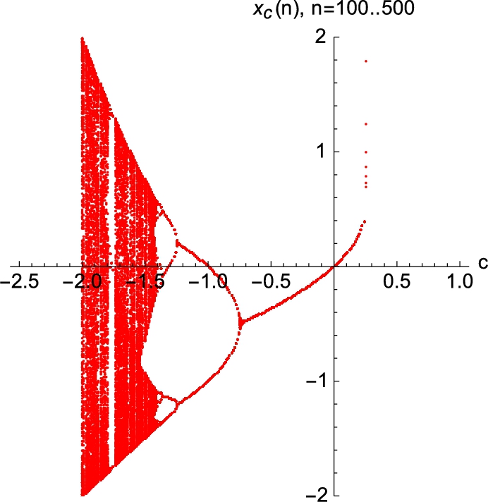
![]()
![]()
![]()
![]() □
□
4.2.1 More on Graphing Lists; Graphing Lists of Points Using Graphics Primitives
Include the Joined->True option in a ListPlot command to connect successive points with line segments or use ListLinePlot.
Using graphics primitives like Point and Line gives you even more flexibility.
Point[{x,y}] represents a point at ![]() .
.
Line[{{x1,y1},{x2,y2},...,{xn,yn}}]
represents a sequence of points ![]() ,
, ![]() , …,
, …, ![]() connected with line segments. A graphics primitive is declared to be a graphics object with Graphics: Show[Graphics[Point[{x,y}]] displays the point
connected with line segments. A graphics primitive is declared to be a graphics object with Graphics: Show[Graphics[Point[{x,y}]] displays the point ![]() . The advantage of using primitives is that each primitive is affected by the options that directly precede it.
. The advantage of using primitives is that each primitive is affected by the options that directly precede it.
Solution
We begin by entering the data represented in the table as dataunion:
![]()
![]()
![]()
the x-coordinate of each point corresponds to the year, where x is the number of years past 1900, and the y-coordinate of each point corresponds to the percentage of the United States labor force that belonged to unions in the given year. We then use ListPlot to graph the set of points represented in dataunion in lp1, lp2 (illustrating the PlotStyle option), and lp3 (illustrating the PlotJoined option). All three plots are displayed side-by-side in Fig. 4.14 using Show together with GraphicsRow.
![]()
![]()
![]()
![]()
![]()
![]()
![]()
![]()
![]()
![]()
An alternative to using ListPlot is to use Show, Graphics, and Point to view the data represented in dataunion. In the following command we use Map to apply the function Point to each pair of data in dataunion. The result is not a graphics object and cannot be displayed with Show.
![]()
![]()
![]()
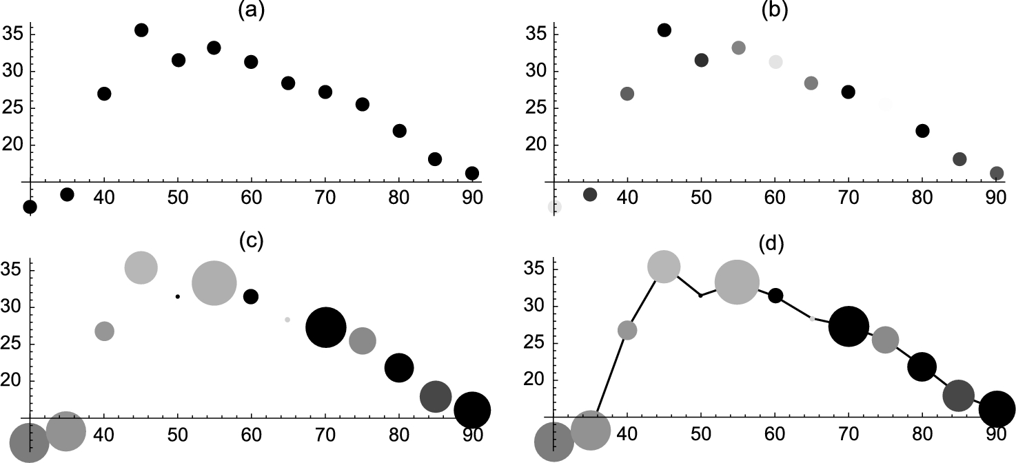
Next, we use Show and Graphics to declare the set of points Map[Point,dataunion] as graphics objects and name the resulting graphics object dp1. The image is not displayed because a semi-colon is included at the end of the command. The PointSize[.03] command specifies that the points be displayed as filled circles of radius ![]() of the displayed graphics object.
of the displayed graphics object.
![]()
![]()
The collection of all commands contained within a Graphics command is contained in braces {...}. Each graphics primitive is affected by the options like PointSize, GrayLevel (or RGBColor) directly preceding it. Thus,
![]()
![]()
![]()
![]()
displays the points in dataunion in various shades of gray in a graphic named dp2 and
![]()
![]()
![]()
![]()
shows the points in dataunion in various sizes and in various shades of gray in a graphic named dp3. We connect successive points with line segments
![]()
![]()
![]()
and show all four plots in Fig. 4.15 using Show and GraphicsGrid.
![]() □
□
With the speed of today's computers and the power of Mathematica, it is relatively easy now to carry out many calculations that required supercomputers and sophisticated programming experience just a few years ago.
Example 4.17
Julia Sets
Plot Julia sets for ![]() if
if ![]() and
and ![]() .
.
Solution
The sets are visualized by plotting the points ![]() for which
for which ![]() is not large in magnitude so we begin by forming our complex grid. Using Table and Flatten, we define complexpts to be a list of 62,500 points of the form
is not large in magnitude so we begin by forming our complex grid. Using Table and Flatten, we define complexpts to be a list of 62,500 points of the form ![]() for 250 equally spaced real values of a between 0 and 8 and 300 equally spaced real values of b between −4 and 4 and then
for 250 equally spaced real values of a between 0 and 8 and 300 equally spaced real values of b between −4 and 4 and then ![]() .
.
![]()
![]()
![]()
![]()
For a given value of ![]() ,
, ![]() returns the ordered triple consisting of the real part of c, the imaginary part of c, and the value of
returns the ordered triple consisting of the real part of c, the imaginary part of c, and the value of ![]() .
.
![]()
We then use Map to apply h to complexpts. Observe that Mathematica generates several error messages. When machine precision is exceeded, we obtain an Overflow[] error message; numerical results smaller than machine precision results in an Underflow[] error message. Error messages can be machine specific, so if you don't get any, don't worry. For length considerations, we don't show any that we obtained here.
![]()
We use the error messages to our advantage. In t2, we select those elements of t1 for which the third coordinate is not Indeterminate, which corresponds to the ordered triples ![]() for which
for which ![]() is not large in magnitude while in t2b, we select those elements of t1 for which the third coordinate is Indeterminate, which corresponds to the ordered triples
is not large in magnitude while in t2b, we select those elements of t1 for which the third coordinate is Indeterminate, which corresponds to the ordered triples ![]() for which
for which ![]() is large in magnitude.
is large in magnitude.
![]()
![]()
![]()
![]()
![]()
which are then graphed with ListPlot and shown side-by-side in Fig. 4.16 using Show and GraphicsRow. As expected, the images are inversions of each other.

 . (University of Iowa colors)
![]()
![]()
![]()
![]()
![]()
Changing λ from 0.66i to 0.665i results in a surprising difference in the plots. We proceed as before but increase the number of sample points to 120,000. See Fig. 4.17.
 .
.
![]()
![]()
![]()
![]()
![]()
![]()
![]()
![]()
![]()
![]()
![]()
![]()
![]()
![]()
![]()
![]()
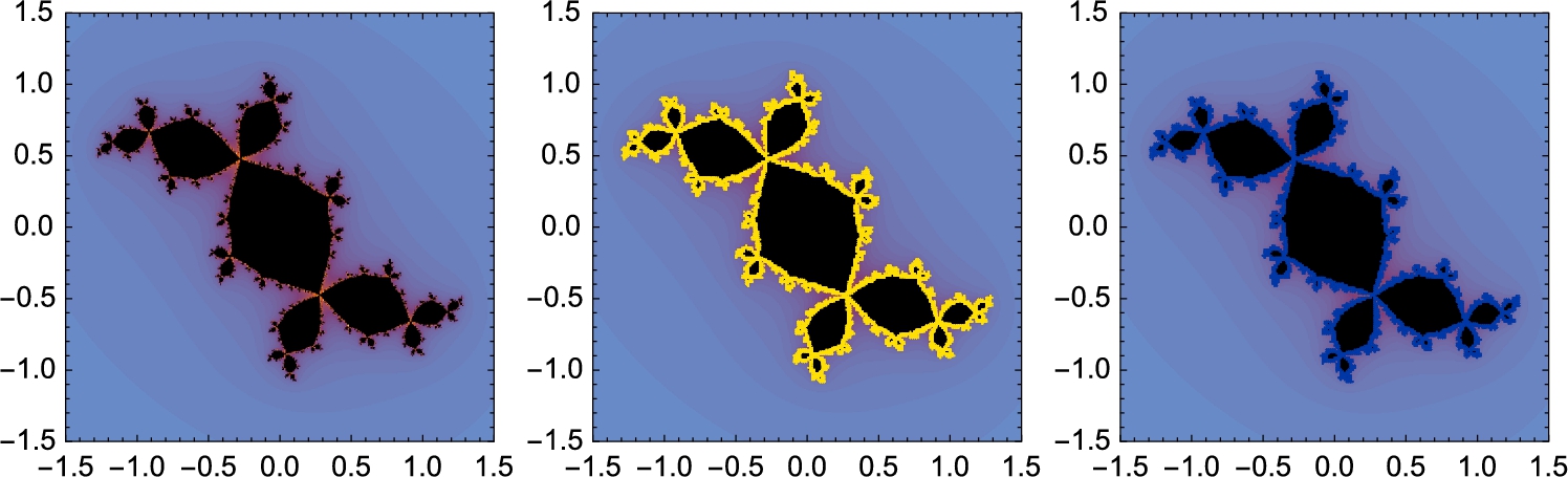
To see detail, we take advantage of pure functions, Map, and graphics primitives in three different ways. In Fig. 4.18, the shading of the point ![]() is assigned according to the distance of
is assigned according to the distance of ![]() from the origin. The color black indicates a distance of zero from the origin; as the distance increases, the shading of the point becomes lighter.
from the origin. The color black indicates a distance of zero from the origin; as the distance increases, the shading of the point becomes lighter.
 .
.
![]()
![]()
![]()
![]()
![]()
![]()
![]()
![]()
![]()
![]()
![]()
![]()
![]()
![]()
![]()
![]()
Often times the Julia set is only defined for a rational function. With Mathematica, the command JuliaSetPlot[f[z],z] plots the Julia set of the rational function ![]() . To obtain good results, you will often want to take advantage of options such as PlotRange and PlotStyle. However, by the nature of the computations involved you should view JuliaSetPlot as a “fragile” commmand.
. To obtain good results, you will often want to take advantage of options such as PlotRange and PlotStyle. However, by the nature of the computations involved you should view JuliaSetPlot as a “fragile” commmand.
To illustrate approximating a Julia set for ![]() , we first use Series together with Normal to compute the Maclaurin series of degree 24 for
, we first use Series together with Normal to compute the Maclaurin series of degree 24 for ![]() . We then use JuliaSetPlot to graph the Julia set for this polynomial in jp1. See Fig. 4.19 (a). Observe that the approximation is fairly close to what we obtained previously.
. We then use JuliaSetPlot to graph the Julia set for this polynomial in jp1. See Fig. 4.19 (a). Observe that the approximation is fairly close to what we obtained previously.
 and .
and .
![]()
![]()
![]()
![]()
On the other hand, when we repeat the approximation process for ![]() , in Fig. 4.19 (b), we see that the approximation does not appear to agree as well as the approximation for
, in Fig. 4.19 (b), we see that the approximation does not appear to agree as well as the approximation for ![]() .
.
![]()
![]()
![]()
![]()
![]() □
□
4.2.2 Miscellaneous List Operations
4.2.2.1 Other List Operations
Some other Mathematica commands used with lists include:
1. Append[list,element], which appends element to list;
2. AppendTo[list,element], which appends element to list and names the result list;
3. Drop[list,n], which returns the list obtained by dropping the first n elements from list;
4. Drop[list,-n], which returns the list obtained by dropping the last n elements of list;
5. Drop[list,{n,m}], which returns the list obtained by dropping the nth through mth elements of list;
6. Drop[list,{n}], which returns the list obtained by dropping the nth element of list;
7. Prepend[list,element], which prepends element to list; and
8. PrependTo[list,element], which prepends element to list and names the result list.
4.2.2.2 Alternative Way to Evaluate Lists by Functions
Abbreviations of several of the commands discussed in this section are summarized in the following table.
| @@ Apply | // (function application) | {...} List |
| /@ Map | [[...]] Part |
4.3 Other Applications
We now present several other applications that we find interesting and require the manipulation of lists. The examples also illustrate (and combine) many of the techniques that were demonstrated in the earlier chapters.
4.3.1 Approximating Lists with Functions
Another interesting application of lists is that of curve-fitting. The commands
1. Fit[data,functionset,variables] fits the list of data points data using the functions in functionset by the method of least-squares. The functions in functionset are functions of the variables listed in variables; and
2. InterpolatingPolynomial[data,x] fits the list of n data points data with an ![]() degree polynomial in the variable x.
degree polynomial in the variable x.
Solution
The approximating function obtained via the least-squares method with Fit is plotted along with the data points in Fig. 4.20. Notice that many of the data points are not very close to the approximating function. A better approximation is obtained using a polynomial of higher degree (4).
![]()
![]()
![]()
![]()
![]()
![]()
![]()
![]()
![]()
![]()
![]()
![]()
![]()
![]()
![]()
To check its accuracy, the second approximation is graphed simultaneously with the data points in Fig. 4.20 (b). □
Next, consider a list of data points made up of ordered pairs.
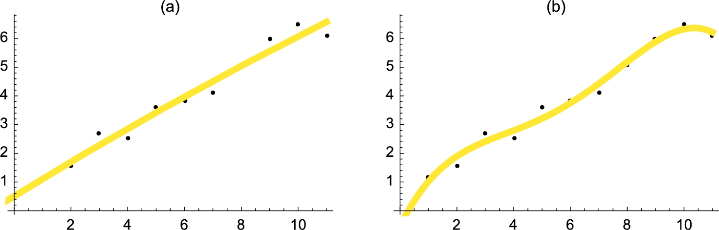
Example 4.19
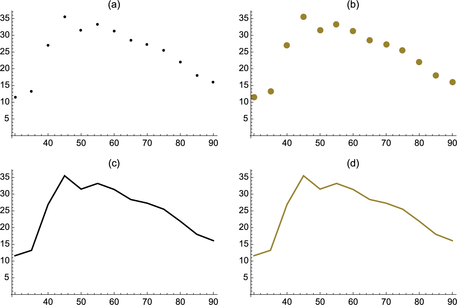
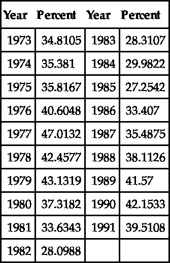
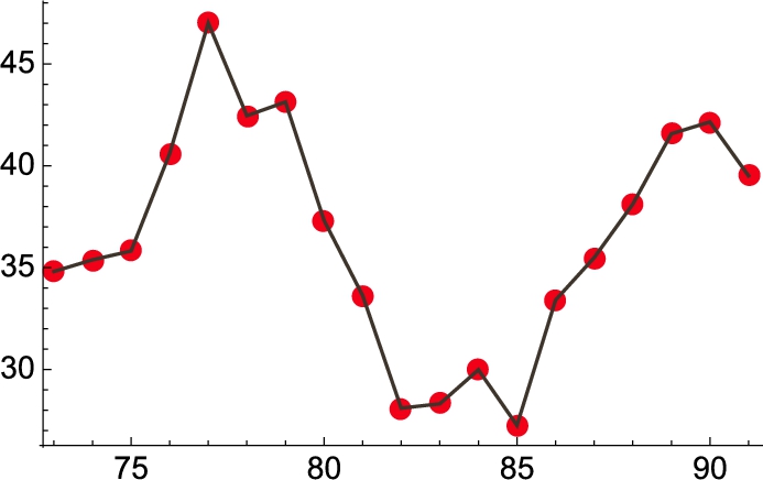
Table 4.2 shows the average percentage of petroleum products imported to the United States for certain years. (a) Graph the points corresponding to the data in the table and connect the consecutive points with line segments. (b) Use InterpolatingPolynomial to find a function that approximates the data in the table. (c) Find a fourth degree polynomial approximation of the data in the table. (d) Find a trigonometric approximation of the data in the table.
Table 4.2
Petroleum Products Imported to the United States for Certain Years
| Year | Percent | Year | Percent |
| 1973 | 34.8105 | 1983 | 28.3107 |
| 1974 | 35.381 | 1984 | 29.9822 |
| 1975 | 35.8167 | 1985 | 27.2542 |
| 1976 | 40.6048 | 1986 | 33.407 |
| 1977 | 47.0132 | 1987 | 35.4875 |
| 1978 | 42.4577 | 1988 | 38.1126 |
| 1979 | 43.1319 | 1989 | 41.57 |
| 1980 | 37.3182 | 1990 | 42.1533 |
| 1981 | 33.6343 | 1991 | 39.5108 |
| 1982 | 28.0988 |
Solution
We begin by defining data to be the set of ordered pairs represented in the table: the x-coordinate of each point represents the number of years past 1900 and the y-coordinate represents the percentage of petroleum products imported to the United States.
![]()
![]()
![]()
![]()
![]()
![]()
We use ListPlot to graph the ordered pairs in data. Note that because the option PlotStyle->PointSize[.03] is included within the ListPlot command, the points are larger than they would normally be. We also use ListPlot with the option PlotJoined->True to graph the set of points data and connect consecutive points with line segments. Then we use Show to display lp1 and lp2 together in Fig. 4.21. Note that in the result, the points are easy to distinguish because of their larger size.
![]()
![]()
![]()
![]()
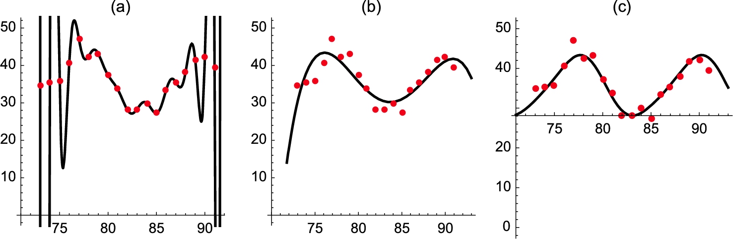
Next, we use InterpolatingPolynomial to find a polynomial approximation, p, of the data in the table. Note that the result is lengthy, so Short is used to display an abbreviated form of p. We then graph p and show the graph of p along with the data in the table for the years corresponding to 1971 to 1993 in Fig. 4.22 (a). Although the interpolating polynomial agrees with the data exactly, the interpolating polynomial oscillates wildly.
![]()
![]()
![]()
![]()
![]()
![]()
To find a polynomial that approximates the data but does not oscillate wildly, we use Fit. Again, we graph the fit and display the graph of the fit and the data simultaneously. In this case, the fit does not identically agree with the data but does not oscillate wildly as illustrated in Fig. 4.22 (b).
![]()
![]()
![]()
![]()
![]()
![]()
![]()
In addition to curve-fitting with polynomials, Mathematica can also fit the data with trigonometric functions. In this case, we use Fit to find an approximation of the data of the form ![]() . As in the previous two cases, we graph the fit and display the graph of the fit and the data simultaneously; the results are shown in Fig. 4.22 (c).
. As in the previous two cases, we graph the fit and display the graph of the fit and the data simultaneously; the results are shown in Fig. 4.22 (c).
![]()
![]()
![]()
![]()
![]()
![]()
![]()
![]()
![]()
![]() □
□
4.3.2 Introduction to Fourier Series
Many problems in applied mathematics are solved through the use of Fourier series. Mathematica assists in the computation of these series in several ways. Suppose that ![]() is defined on
is defined on ![]() . Then the Fourier series for
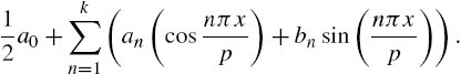
. Then the Fourier series for ![]() is
is
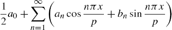
where
The kth term of the Fourier series (4.1) is
The kth partial sum of the Fourier series (4.1) is
It is a well-known theorem that if ![]() is a periodic function with period 2p and
is a periodic function with period 2p and ![]() is continuous on
is continuous on ![]() except at finitely many points, then at each point x the Fourier series for
except at finitely many points, then at each point x the Fourier series for ![]() converges and
converges and

In fact, if the series ![]() converges, then the Fourier series converges uniformly on
converges, then the Fourier series converges uniformly on ![]() .
.
In the special case that ![]() , FourierSeries, FourierCosSeries, and FourierSinSeries can be used to carry out these calculations. If
, FourierSeries, FourierCosSeries, and FourierSinSeries can be used to carry out these calculations. If ![]() is defined on
is defined on ![]() , FourierSeries[f[x],x,n] finds the first n terms of the Fourier series for
, FourierSeries[f[x],x,n] finds the first n terms of the Fourier series for ![]() , FourierCosSeries[f[x],x,n] finds the first n terms of the Fourier cosine series for
, FourierCosSeries[f[x],x,n] finds the first n terms of the Fourier cosine series for ![]() (even extension), and FourierSinSeries[f[x],x,n] finds the first n terms of the Fourier sin series for
(even extension), and FourierSinSeries[f[x],x,n] finds the first n terms of the Fourier sin series for ![]() (odd extension).
(odd extension).
Example 4.20
Let 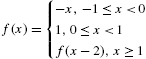 . Compute and graph the first few partial sums of the Fourier series for
 ![]() .
.
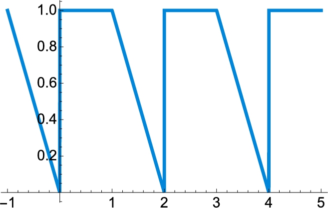
We begin by clearing all prior definitions of f. We then define the piecewise function ![]() and graph
and graph ![]() on the interval
on the interval ![]() in Fig. 4.23.
in Fig. 4.23.
![]()
![]()
![]()
![]()
![]()
![]()
The Fourier series coefficients are computed with the integral formulas in equation (4.2). Executing the following commands defines p to be 1, a[0] to be an approximation of the integral ![]() , a[n] to be an approximation of the integral
, a[n] to be an approximation of the integral ![]() , and b[n] to be an approximation of the integral
, and b[n] to be an approximation of the integral ![]() .
.
![]()
![]()
![]()
0.75
![]()
![]()
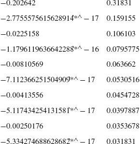
A table of the coefficients a[i] and b[i] for ![]() , 2, 3, …, 10 is generated with Table and named coeffs. Several error messages (which are not displayed here for length considerations) are generated because of the discontinuities but the resulting approximations are satisfactory for our purposes. The elements in the first column of the table represent the
, 2, 3, …, 10 is generated with Table and named coeffs. Several error messages (which are not displayed here for length considerations) are generated because of the discontinuities but the resulting approximations are satisfactory for our purposes. The elements in the first column of the table represent the ![]() 's and the second column represents the
's and the second column represents the ![]() 's. Notice how the elements of the table are extracted using double brackets with coeffs.
's. Notice how the elements of the table are extracted using double brackets with coeffs.
![]()
![]()
The first element of the list is extracted with coeffs[[1]].
![]()
![]()
The first element of the second element of coeffs and the second element of the third element of coeffs are extracted with coeffs[[2,1]] and coeffs[[3,2]], respectively.
![]()
![]()
![]()
0.106103
After the coefficients are calculated, the nth partial sum of the Fourier series is obtained with Sum. The kth term of the Fourier series, ![]() , is defined in fs. Hence, the nth partial sum of the series is given by
, is defined in fs. Hence, the nth partial sum of the series is given by
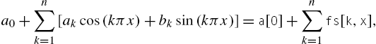
which is defined in fourier using Sum. We illustrate the use of fourier by finding fourier[2,x] and fourier[3,x].
![]()
![]()
![]()
![]()
![]()
![]()
To see how the Fourier series approximates the periodic function, we plot the function simultaneously with the Fourier approximation for ![]() and
and ![]() . The results are displayed together using GraphicsArray in Fig. 4.24.
. The results are displayed together using GraphicsArray in Fig. 4.24.

![]()
![]()
![]()
![]()
![]()
![]()
![]() □
□
Example 4.21
For the first five terms of the Fourier series, Fourier cosine series, and Fourier sine series for ![]() on
on ![]() .
.
Solution
Here we use FourierSeries, FourierCosSeries, and FourierSinSeries.
![]()
![]()
![]()
![]()
![]()
![]()
![]()
![]()
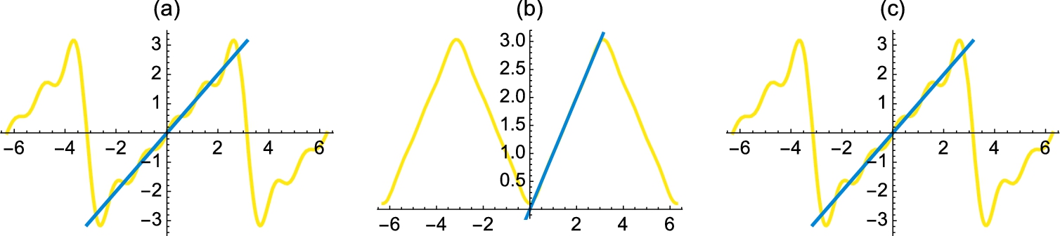
Next, we graph the Fourier approximations with ![]() in Fig. 4.25. In the figure, observe that the Fourier series is the periodic extension of
in Fig. 4.25. In the figure, observe that the Fourier series is the periodic extension of ![]() , the Fourier cosine series is the even periodic extension of
, the Fourier cosine series is the even periodic extension of ![]() , and the Fourier sine series is the odd periodic extension of
, and the Fourier sine series is the odd periodic extension of ![]() .
.
![]()
![]()
![]()
![]()
![]()
![]()
![]()
![]()
![]()
![]() □
□
Application: The One-Dimensional Heat Equation
A typical problem in applied mathematics that involves the use of Fourier series is that of the one-dimensional heat equation. The boundary value problem that describes the temperature in a uniform rod with insulated surface is
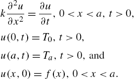
In this case, the rod has “fixed end temperatures” at ![]() and
and ![]() and
and ![]() is the initial temperature distribution. The solution to the problem is
is the initial temperature distribution. The solution to the problem is
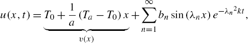
where

and is obtained through separation of variables techniques. The coefficient ![]() in the solution equation (4.6) is the Fourier series coefficient
in the solution equation (4.6) is the Fourier series coefficient ![]() of the function
of the function ![]() , where
, where ![]() is the steady-state temperature.
is the steady-state temperature.
Example 4.22
Solve 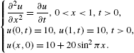
Solution
In this case, ![]() and
and ![]() . The fixed end temperatures are
. The fixed end temperatures are ![]() , and the initial heat distribution is
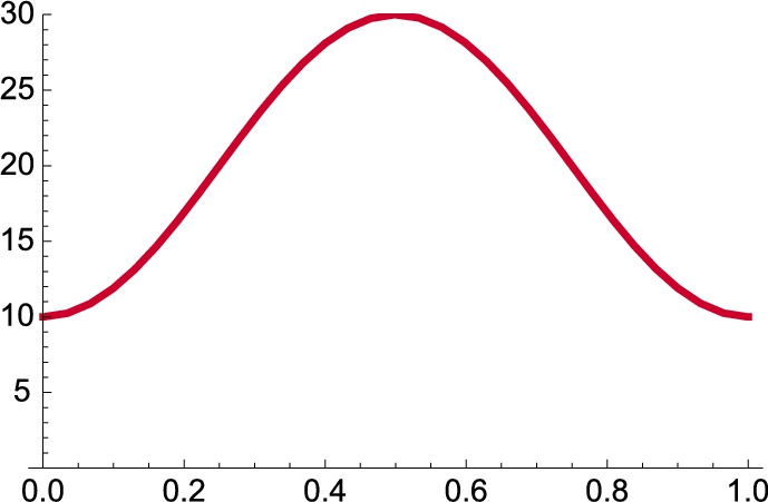
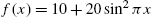
, and the initial heat distribution is ![]() . The steady-state temperature is
. The steady-state temperature is ![]() . The function
. The function ![]() is defined and plotted in Fig. 4.26. Also, the steady-state temperature,
is defined and plotted in Fig. 4.26. Also, the steady-state temperature, ![]() , and the eigenvalue are defined. Finally, Integrate is used to define a function that will be used to calculate the coefficients of the solution.
, and the eigenvalue are defined. Finally, Integrate is used to define a function that will be used to calculate the coefficients of the solution.
 . (University of Utah colors)
![]()
![]()
![]()
![]()
![]()
![]()
![]()
Notice that b[n] is defined using the form b[n_]:=b[n]=... so that Mathematica “remembers” the values of b[n] computed and thus avoids recomputing previously computed values. In the following table, we compute exact and approximate values of b[1],...,b[10].
![]()
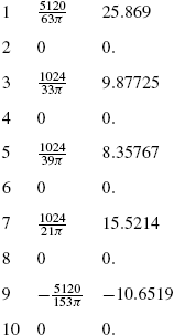
Let ![]() . Then, the desired solution,
. Then, the desired solution, ![]() , is given by
, is given by
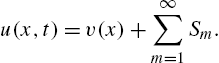
Let ![]() . Notice that
. Notice that ![]() . Consequently, approximations of the solution to the heat equation are obtained recursively taking advantage of Mathematica's ability to compute recursively. The solution is first defined for
. Consequently, approximations of the solution to the heat equation are obtained recursively taking advantage of Mathematica's ability to compute recursively. The solution is first defined for ![]() by u[x,t,1]. Subsequent partial sums, u[x,t,n], are obtained by adding the nth term of the series,
by u[x,t,1]. Subsequent partial sums, u[x,t,n], are obtained by adding the nth term of the series, ![]() , to u[x,t,n-1].
, to u[x,t,n-1].
![]()
![]()
By defining the solution in this manner a table can be created that includes the partial sums of the solution. In the following table, we compute the first, fourth, and seventh partial sums of the solution to the problem. (See Fig. 4.27.)
![]()
![]()
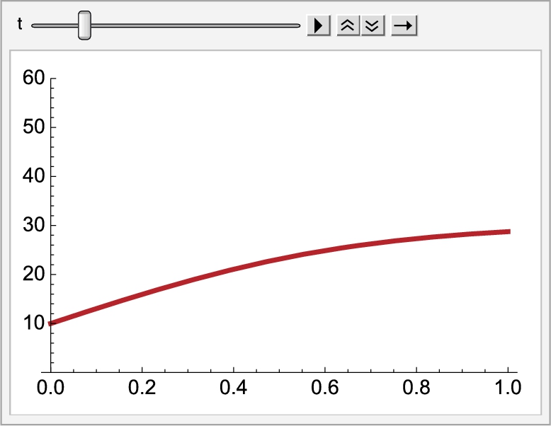
To generate graphics that can be animated, we use Animate. The 10th partial sum of the solution is plotted for ![]() to
to ![]() .
.
![]()
![]()
![]()
Alternatively, we may generate several graphics and display the resulting set of graphics as a GraphicsArray. We plot the 10th partial sum of the solution for ![]() to
to ![]() using a step-size of 1/15. The resulting 16 graphs are named graphs which are then partitioned into four element subsets with Partition and named toshow. We then use Show and GraphicsGrid to display toshow in Fig. 4.28.
using a step-size of 1/15. The resulting 16 graphs are named graphs which are then partitioned into four element subsets with Partition and named toshow. We then use Show and GraphicsGrid to display toshow in Fig. 4.28.
![]()
![]()
![]()
![]() □
□
Fourier series and generalized Fourier series arise in too many applications to list. Examples using them illustrate Mathematica's power to manipulate lists, symbolics, and graphics.
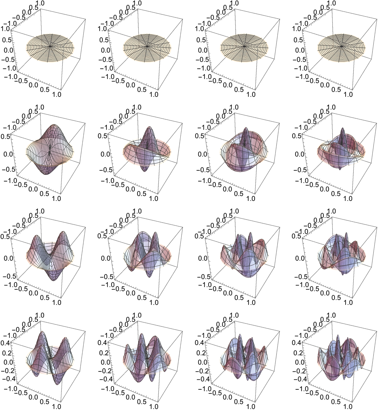
Application: The Wave Equation on a Circular Plate
The vibrations of a circular plate satisfy the equation
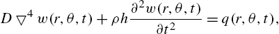
where ![]() and
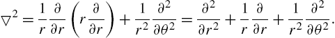
and ![]() is the Laplacian in polar coordinates, which is defined by
is the Laplacian in polar coordinates, which is defined by
Assuming no forcing so that ![]() and
and ![]() , equation (4.7) can be written as
, equation (4.7) can be written as
For a clamped plate, the boundary conditions are ![]() and after much work (see [7]) the normal modes are found to be
and after much work (see [7]) the normal modes are found to be
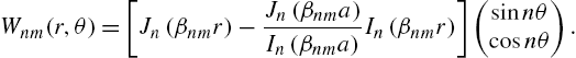
In equation (4.9), ![]() where
where ![]() is the mth solution of
is the mth solution of
where ![]() is the Bessel function of the first kind of order n and
is the Bessel function of the first kind of order n and ![]() is the modified Bessel function of the first kind of order n, related to
is the modified Bessel function of the first kind of order n, related to ![]() by
by ![]() .
.
The Mathematica command BesselI[n,x] returns ![]() .
.
Solution
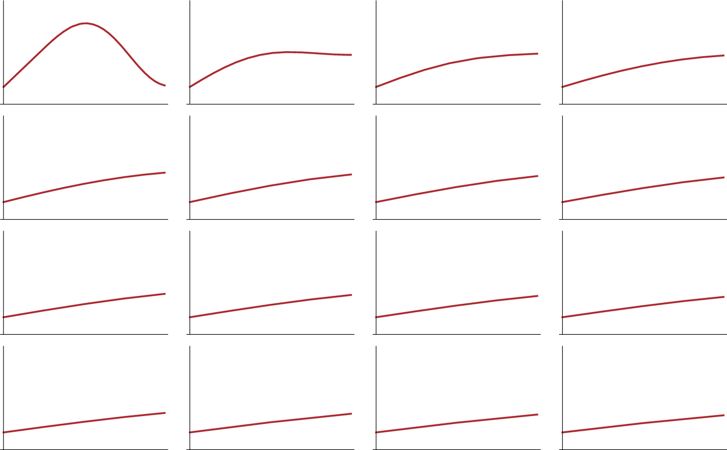
We must determine the value of ![]() for several values of n and m so we begin by defining eqn[n][x] to be
for several values of n and m so we begin by defining eqn[n][x] to be ![]() . The mth solution of equation (4.10) corresponds to the mth zero of the graph of eqn[n][x] so we graph eqn[n][x] for
. The mth solution of equation (4.10) corresponds to the mth zero of the graph of eqn[n][x] so we graph eqn[n][x] for ![]() , 1, 2, and 3 with Plot in Fig. 4.29.
, 1, 2, and 3 with Plot in Fig. 4.29.
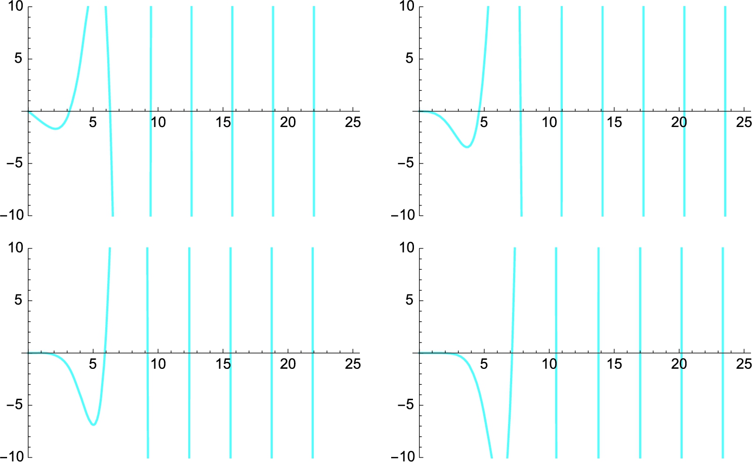
 for n = 0 and 1 in the first row; n = 2 and 3 in the second row.
![]()
The result of the Table and Plot command is a list of length four, which is verified with Length[p1].
![]()
![]()
so we use Partition to create a ![]() array of graphics which is displayed using Show and GraphicsGrid.
array of graphics which is displayed using Show and GraphicsGrid.
![]()
To determine ![]() we use FindRoot. Recall that to use FindRoot to solve an equation an initial approximation of the solution must be given. For example,
we use FindRoot. Recall that to use FindRoot to solve an equation an initial approximation of the solution must be given. For example,
![]()
![]()
approximates ![]() , the first solution of equation (4.10) if
, the first solution of equation (4.10) if ![]() . However, the result of FindRoot is a list. The specific value of the solution is the second part of the first part of the list, l01, extracted from the list with Part ([[...]]).
. However, the result of FindRoot is a list. The specific value of the solution is the second part of the first part of the list, l01, extracted from the list with Part ([[...]]).
![]()
3.19622
Thus,
![]()
![]()
approximates the first five solutions of equation (4.10) if ![]() and then returns the specific value of each solution. We use the same steps to approximate the first five solutions of equation (4.10) if
and then returns the specific value of each solution. We use the same steps to approximate the first five solutions of equation (4.10) if ![]() , 2, and 3.
, 2, and 3.
![]()
![]()
![]()
![]()
![]()
![]()
All four lists are combined together in λs.
![]()
![]()
![]()
For ![]() , 1, 2, and 3 and
, 1, 2, and 3 and ![]() , 2, 3, 4, and 5,
, 2, 3, 4, and 5, ![]() is the mth part of the
is the mth part of the ![]() st part of λs.
st part of λs.
Observe that the value of a does not affect the shape of the graphs of the normal modes so we use ![]() and then define
and then define ![]() .
.
![]()
![]()
ws is defined to be the sine part of equation (4.9)
![]()
![]()
![]()
and wc to be the cosine part.
![]()
![]()
![]()
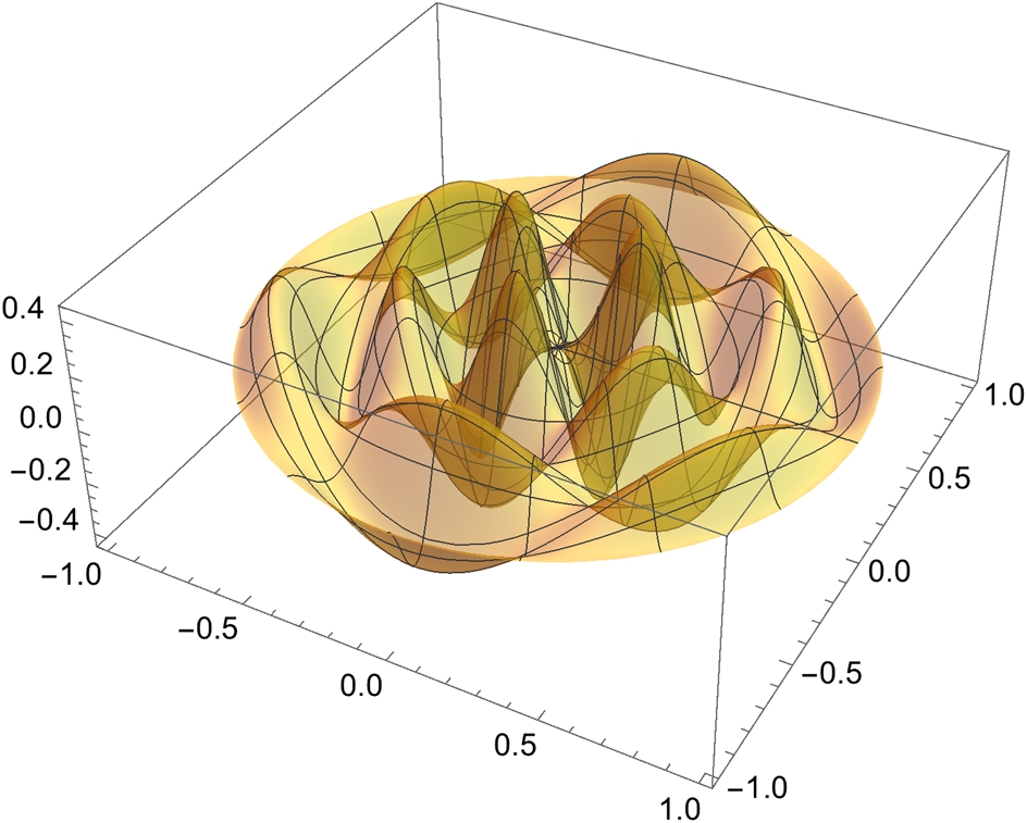
We use ParametricPlot3D to plot ws and wc. For example,
![]()
![]()
graphs the sine part of ![]() shown in Fig. 4.30.
shown in Fig. 4.30.
We use Table together with ParametricPlot3D followed by Show and GraphicsGrid to graph the sine part of ![]() for
for ![]() , 1, 2, and 3 and
, 1, 2, and 3 and ![]() , 2, 3, and 4 shown in Fig. 4.31.
, 2, 3, and 4 shown in Fig. 4.31.
![]()
![]()
![]()
![]()
Identical steps are followed to graph the cosine part shown in Fig. 4.32.

![]()
![]()
![]()
![]() □
□
4.3.3 The Mandelbrot Set and Julia Sets
In Examples 4.9, 4.15, and 4.17 we illustrated several techniques for plotting bifurcation diagrams and Julia sets. For investigating Julia sets, try using built-in commands like JuliaSetPlot first. Similarly, for investigating the Mandelbrot set, try MandelbrotSetPlot along with its many options to see if you can obtain your desired results before spending a lot of time writing your own code.
Let ![]() . In Example 4.15, we generated the c-values when plotting the bifurcation diagram of
. In Example 4.15, we generated the c-values when plotting the bifurcation diagram of ![]() . Depending upon how you think and approach various problems, some approaches may be easier to understand than others. With the exception of very serious calculations, the differences in the time needed to carry out the computations may be minimal so we encourage you to follow the approach that you understand.
. Depending upon how you think and approach various problems, some approaches may be easier to understand than others. With the exception of very serious calculations, the differences in the time needed to carry out the computations may be minimal so we encourage you to follow the approach that you understand.
![]() is the special case of
is the special case of ![]() for
for ![]() .
.
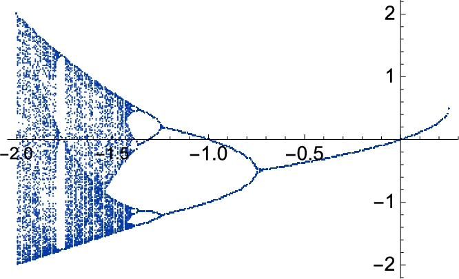
Example 4.24
Dynamical Systems
For example, entering
![]()
![]()
defines ![]() so
so
![]()
![]()
computes ![]() and
and
![]()
![]()
returns a list of ![]() for
for ![]() , 102, …, 200. Thus,
, 102, …, 200. Thus,
![]()
![]()
![]()
300
returns a list of lists of ![]() for
for ![]() , 102, …, 200 for 300 equally spaced values of c between −2 and 1. The list lgtable is converted to a list of points with Flatten and plotted with ListPlot. See Fig. 4.33 and compare this result to the result obtained in Example 4.15.
, 102, …, 200 for 300 equally spaced values of c between −2 and 1. The list lgtable is converted to a list of points with Flatten and plotted with ListPlot. See Fig. 4.33 and compare this result to the result obtained in Example 4.15.
![]()
![]()
![]()
For a given complex number c the Julia set, ![]() , of
, of ![]() is the set of complex numbers,
is the set of complex numbers, ![]() ,
, ![]() real, for which the sequence z,
real, for which the sequence z, ![]() ,
, ![]() , …,
, …, ![]() , …, does not tend to ∞ as
, …, does not tend to ∞ as ![]() :
:
Using a dynamical system, setting ![]() and computing
and computing ![]() for large n can help us determine if z is an element of
for large n can help us determine if z is an element of ![]() . In terms of a composition, computing
. In terms of a composition, computing ![]() for large n can help us determine if z is an element of
for large n can help us determine if z is an element of ![]() .
.
We use the notation ![]() to represent the composition
to represent the composition ![]() .
.
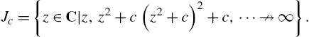
Example 4.25
Julia Sets
Plot the Julia set of ![]() if
if ![]() .
.
Solution
After defining ![]() , we use Table together with Nest to compute ordered triples of the form
, we use Table together with Nest to compute ordered triples of the form ![]() for 150 equally spaced values of x between
for 150 equally spaced values of x between ![]() and 3/2 and 150 equally spaced values of y between
and 3/2 and 150 equally spaced values of y between ![]() and 3/2.
and 3/2.
You do not need to redefine ![]() if you have already defined it during your current Mathematica session.
if you have already defined it during your current Mathematica session.
![]()
![]()
![]()
![]()
![]()
![]()
![]()
We remove those elements of g2 for which the third coordinate is Overflow[] with Select,
![]()
extract a list of the first two coordinates, ![]() , from the elements of g3,
, from the elements of g3,
![]()
and plot the resulting list of points in Fig. 4.34 using ListPlot.
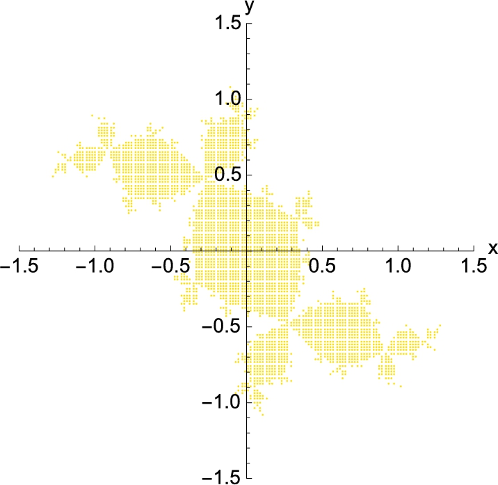
![]()
![]()
![]()
We can invert the image as well with the following commands. In the end result, we show the Julia set and its inverted image in Fig. 4.35

![]()
![]()
![]()
![]()
![]()
For rational functions ![]() you can use the command JuliaSetPlot[f[z],z] to plot the Julia set for
you can use the command JuliaSetPlot[f[z],z] to plot the Julia set for ![]() . The default is
. The default is ![]() so JuliaSetPlot[c] plots the Julia set for
so JuliaSetPlot[c] plots the Julia set for ![]() . Use options like PlotRange to get the view of the plot that you expect.
. Use options like PlotRange to get the view of the plot that you expect.
Thus, in the following commands, all plot the Julia set for ![]() for
for ![]() .
.
![]()
![]()
![]()
![]()
![]()
![]()
![]()
The plots are all shown together in Fig. 4.36.
![]() □
□
Of course, one can consider functions other than ![]() as well as rearrange the order in which we carry out the computations.
as well as rearrange the order in which we carry out the computations.
Example 4.26
Julia Sets
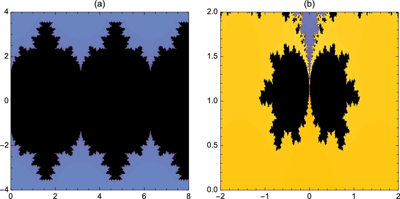
Plot the Julia set for ![]() if
if ![]() .
.
Solution
Observe that ![]() is a true rational function (it is a polynomial) so JuliaSetPlot will plot the Julia set.
is a true rational function (it is a polynomial) so JuliaSetPlot will plot the Julia set.
After defining ![]() ,
,
![]()
![]()
we use JuliaSetPlot as in the previous example. See Fig. 4.37.
 .
.
![]()
![]()
You can use commands like Table and Manipulate to investigate the Julia set for ![]() . For example,
. For example,
![]()
![]()
![]()
plots the Julia set for ![]() for 9 equally spaced values of k between .5 and 1.5. The results are shown as an array with GraphicsGrid in Fig. 4.38. □
for 9 equally spaced values of k between .5 and 1.5. The results are shown as an array with GraphicsGrid in Fig. 4.38. □
Example 4.27
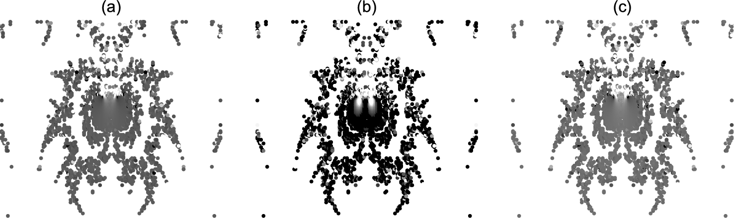
The Ikeda Map
Solution
The basins of attraction for F are the set of points ![]() for which
for which ![]() as
as ![]() .
.
After defining ![]() to be equation (4.11) and then
to be equation (4.11) and then ![]() ,
, ![]() , and
, and ![]() , we use Table followed by Flatten to define pts to be the list of 40,000 ordered pairs
, we use Table followed by Flatten to define pts to be the list of 40,000 ordered pairs ![]() for 200 equally spaced values of x between −2.3 and 1.3 and 200 equally spaced values of y between −2.8 and .8.
for 200 equally spaced values of x between −2.3 and 1.3 and 200 equally spaced values of y between −2.8 and .8.
![]()
![]()
![]()
![]()
![]()
![]()
In l1, we use Map to compute ![]() for each
for each ![]() in pts. In pts2, we use the graphics primitive Point and shade the points according to the maximum value of
in pts. In pts2, we use the graphics primitive Point and shade the points according to the maximum value of ![]() – those
– those ![]() for which
for which ![]() is closest to the origin are darkest; the point
is closest to the origin are darkest; the point ![]() is shaded lighter as the distance of
is shaded lighter as the distance of ![]() from the origin increases. (See Fig. 4.39 (a).)
from the origin increases. (See Fig. 4.39 (a).)

![]()
![]()
![]()
![]()
4.33321
![]()
![]()
![]()
For ![]() , we proceed in the same way. The final results are shown in Fig. 4.39 (b).
, we proceed in the same way. The final results are shown in Fig. 4.39 (b).
![]()
![]()
![]()
4.48421
![]()
![]()
![]()
![]() □
□
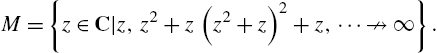
The Mandelbrot set, M, is the set of complex numbers, ![]() ,
, ![]() real, for which the sequence z,
real, for which the sequence z, ![]() ,
, ![]() , …,
, …, ![]() , …, does not tend to ∞ as
, …, does not tend to ∞ as ![]() :
:
Using a dynamical system, setting ![]() and computing
and computing ![]() for large n can help us determine if z is an element of M. In terms of a composition, computing
for large n can help us determine if z is an element of M. In terms of a composition, computing ![]() for large n can help us determine if z is an element of M.
for large n can help us determine if z is an element of M.
The command
MandelbrotSetPlot[{a+bi,c+di}]
plots the Mandelbrot set on the rectangle with lower left corner ![]() and upper right corner
and upper right corner ![]() .
.
Solution
We use MandelbrotSetPlot. The following gives us the image on the left in Fig. 4.40.
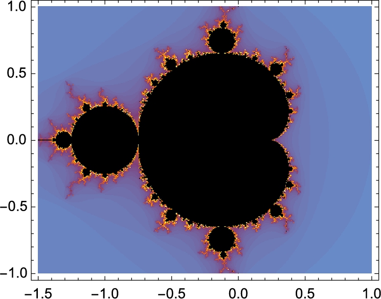
![]() □
□
The Mandelbrot set can be obtained (or more precisely, approximated) by repeatedly composing ![]() for a grid of z-values and then deleting those for which the values exceed machine precision or other specified “large” value. Those values greater than $MaxNumber result in an Overflow[] message; computations with Overflow[] result in an Indeterminate message.
for a grid of z-values and then deleting those for which the values exceed machine precision or other specified “large” value. Those values greater than $MaxNumber result in an Overflow[] message; computations with Overflow[] result in an Indeterminate message.
We can generalize by considering exponents other than 2 by letting ![]() . The generalized Mandelbrot set,
. The generalized Mandelbrot set, ![]() , is the set of complex numbers,
, is the set of complex numbers, ![]() ,
, ![]() real, for which the sequence z,
real, for which the sequence z, ![]() ,
, ![]() , …,
, …, ![]() , …, does not tend to ∞ as
, …, does not tend to ∞ as ![]() :
:
Using a dynamical system, setting ![]() and computing
and computing ![]() for large n can help us determine if z is an element of
for large n can help us determine if z is an element of ![]() . In terms of a composition, computing
. In terms of a composition, computing ![]() for large n can help us determine if z is an element of
for large n can help us determine if z is an element of ![]() .
.
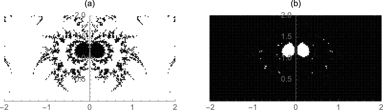
Example 4.29
Generalized Mandelbrot Set
After defining ![]() , we use Table, Abs, and Nest to compute a list of ordered triples of the form
, we use Table, Abs, and Nest to compute a list of ordered triples of the form ![]() for p-values from 1.625 to 2.625 spaced by equal values of 1/8 and 200 values of x (y) values equally spaced between −2 and 2, resulting in 40,000 sample points of the form
for p-values from 1.625 to 2.625 spaced by equal values of 1/8 and 200 values of x (y) values equally spaced between −2 and 2, resulting in 40,000 sample points of the form ![]() .
.
![]()
![]()
![]()
![]()
![]()
![]()
Next, we extract those points for which the third coordinate is Indeterminate with Select, ordered pairs of the first two coordinates are obtained in g4. The resulting list of points is plotted with ListPlot in Fig. 4.41.
![]()
![]()
![]()
![]()
![]()
![]()
More detail is observed if you use the graphics primitive Point as shown in Fig. 4.42. In this case, those points ![]() for which
for which ![]() is small are shaded according to a darker GrayLevel than those points for which
is small are shaded according to a darker GrayLevel than those points for which ![]() is large.
is large.
 is large are shaded lighter than those for which is small.
![]()
![]()
![]()
![]()
![]()
Throughout these examples, we have typically computed the iteration ![]() for “large” n like values of n between 100 and 200. To indicate why we have selected those values of n, we revisit the Mandelbrot set plotted in Example 4.28.
for “large” n like values of n between 100 and 200. To indicate why we have selected those values of n, we revisit the Mandelbrot set plotted in Example 4.28.
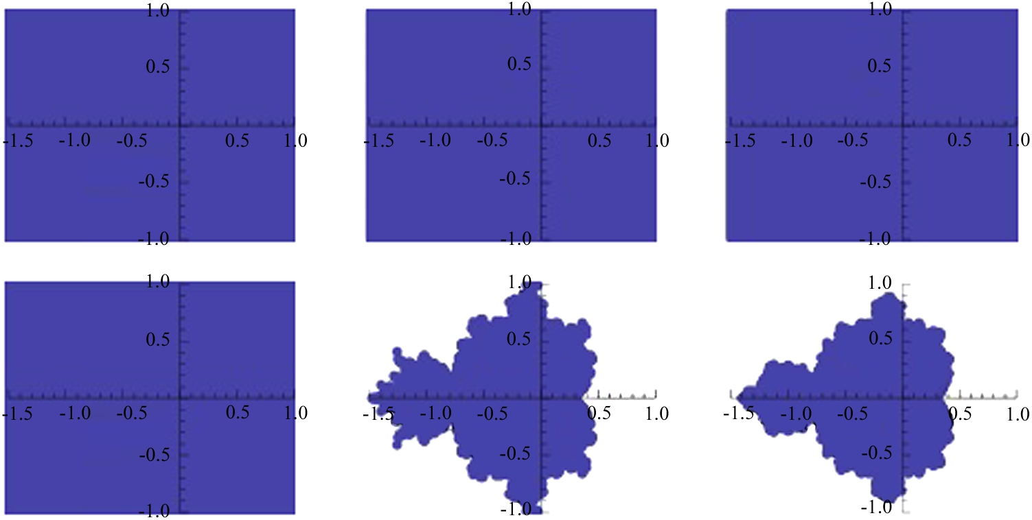
Example 4.30
Mandelbrot Set
We proceed in essentially the same way as in the previous examples. After defining ![]() ,
,
![]()
![]()
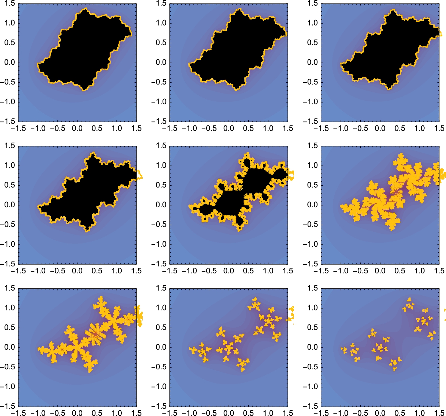
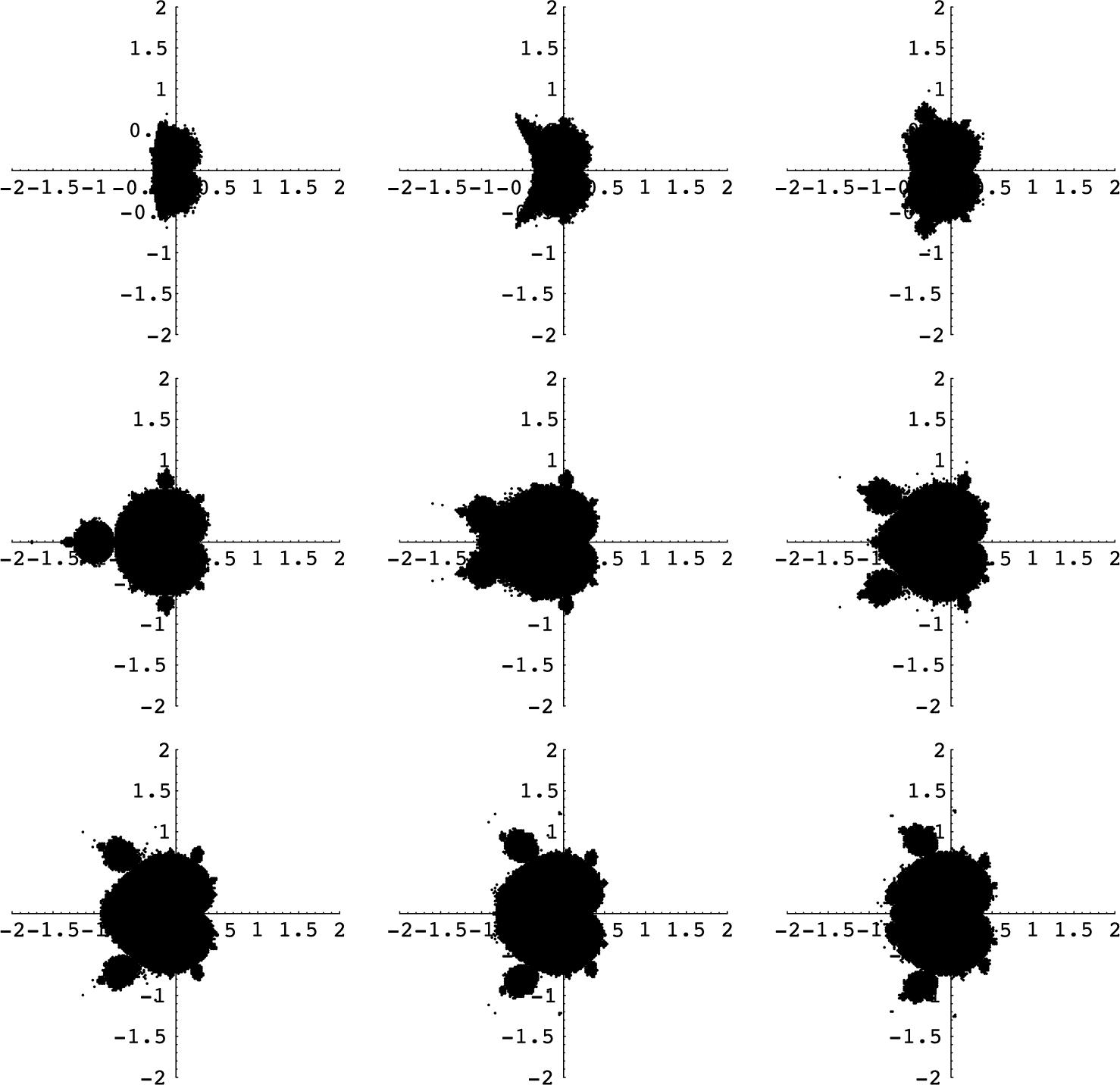
we use Table followed by Map to create a nested list. For each ![]() , 10, 15, 25, 50, and 100, a nested list is formed for 200 equally spaced values of y between −1 and 1 and then 200 equally spaced values of x between −1.5 and 1. between −1.5 and 1. At the bottom level of each nested list, the elements are of the form
, 10, 15, 25, 50, and 100, a nested list is formed for 200 equally spaced values of y between −1 and 1 and then 200 equally spaced values of x between −1.5 and 1. between −1.5 and 1. At the bottom level of each nested list, the elements are of the form ![]() .
.
![]()
![]()
![]()
![]()
![]()
For each value of n, the corresponding list of ordered triples ![]() is obtained using Flatten.
is obtained using Flatten.
![]()
We then remove those points for which the third coordinate, ![]() , is Overflow[] (corresponding to ∞),
, is Overflow[] (corresponding to ∞),
![]()
![]()
extract ![]() from the remaining ordered triples,
from the remaining ordered triples,
![]()
![]()
and graph the resulting sets of points using ListPlot in Fig. 4.43. As shown in Fig. 4.43, we see that Mathematica's numerical precision (and consequently decent plots) are obtained when ![]() or
or ![]() .
.
![]()
![]()
![]()
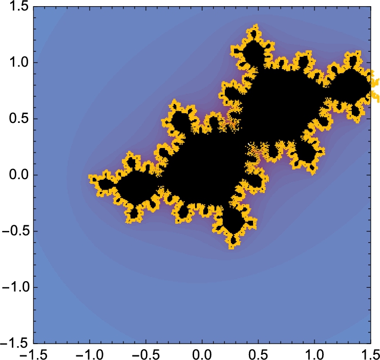
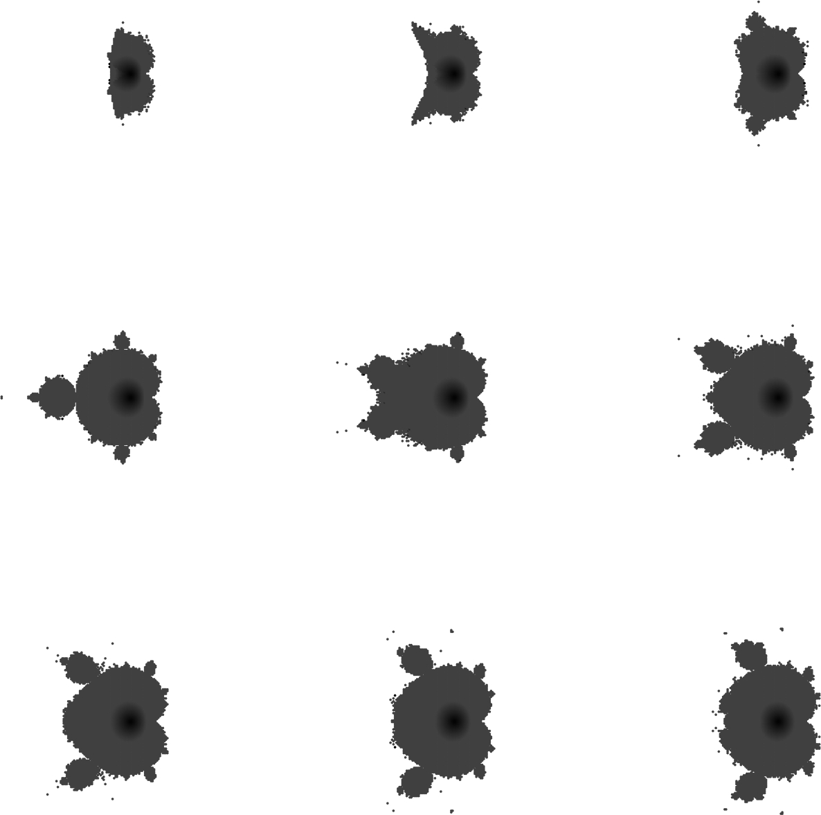
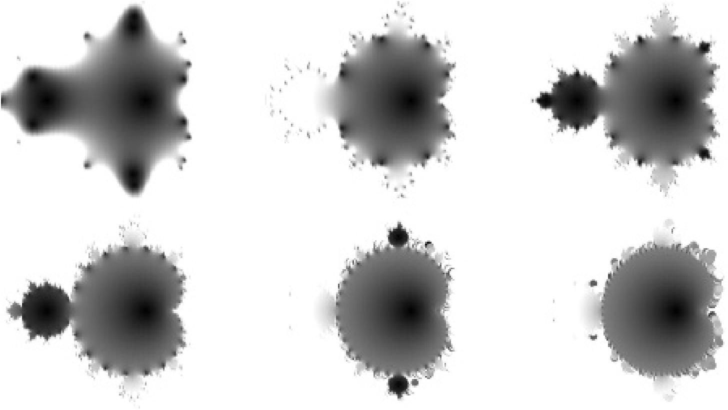
If instead, we use graphics primitives like Point and then shade each point ![]() according to
according to ![]() detail emerges quickly as shown in Fig. 4.44.
detail emerges quickly as shown in Fig. 4.44.
![]()
![]()
![]()
![]()
![]()
The examples like the ones illustrated here indicate that similar results could have been accomplished using far smaller values of n than ![]() or
or ![]() . With fast machines, the differences in the time needed to perform the calculations is minimal;
. With fast machines, the differences in the time needed to perform the calculations is minimal; ![]() and
and ![]() appear to be a “safe” large value of n for well-studied examples like these.
appear to be a “safe” large value of n for well-studied examples like these.