Chapter 14: Subsetting and Combining SAS Data Sets
This chapter discusses ways to subset (filter) a SAS data set and to combine data from several SAS data sets. For those readers who understand SQL (structured query language), you should know that SAS supports SQL in PROC SQL. Because SQL is covered elsewhere in many texts, this chapter does not include a discussion of PROC SQL. The methods described in this chapter, SET, MERGE, and UPDATE, are DATA step statements that provide an alternative to PROC SQL.
Subsetting (Filtering) Data in a SAS Data Set
As you saw in the first section of this book, you can subset or filter a SAS data set using interactive point-and-click operations provided by SAS Studio. This section shows you how to subset a SAS data set using DATA step programming.
To demonstrate how to create a subset starting with observations from an existing SAS data set, let’s use one of the built-in data sets that comes with SAS Studio. There is a library called SASHELP that ships with SAS Studio and contains many data sets to be used for training.
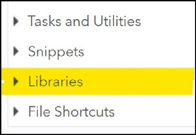
To see a list of data sets in this library, perform the following steps: First, click the Libraries tab in the SAS Studio window.
Figure 14.1: Select the Libraries Tab
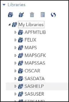
After you click the Libraries tab, select My Libraries and you will then see a list of libraries. (Note: your list might differ slightly from the list in Figure 14.2.)
Figure 14.2: Opening the Libraries Tab
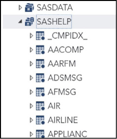
If you click the triangle to the left of SASHELP, you will see a list of all the built-in data sets. A partial list looks like this:
Figure 14.3: Partial list of SASHELP Data Sets
We are going to select the Retail data set. Scroll down the list of data sets and select (double click) RETAIL.
Figure 14.4: Opening the Retail Data Set
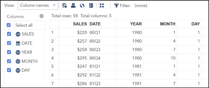
You see the variables in this data set along with a listing of the data set.
Suppose your goal is to concentrate on data from the year 1980. You proceed as follows:
Program 14.1: Using a WHERE Statement to Subset a SAS Data Set
data Year1980;
   set SASHELP.Retail;
   where Year = 1980;
run;

title “Listing of Data Set Year1980”;
proc print data=Year1980 noobs;
run;
You use a SET statement to read the observations in data set SASHELP.Retail. Notice that you do not need to submit a LIBNAME statement. The SASHELP library is automatically made available to you every time you open SAS Studio. To subset the observations in data set Retail, you use a WHERE statement. Following the keyword WHERE, you specify the subsetting condition. In this example, you specify that you only want to see data for the year 1980. Using PROC PRINT, you obtain the following listing:
Figure 14.5: Output from Program 14.1
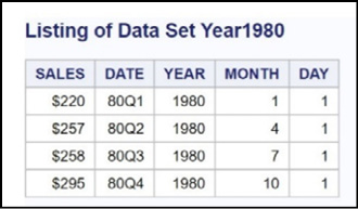
Only four observations met your selection criteria.
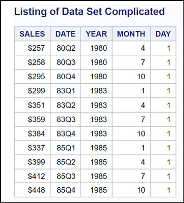
Let’s look at a more complicated subset. Suppose you want data for the years 1980, 1982, and 1985, and you only want to look at observations where the Sales were greater than or equal to $250. Here is the program.
Program 14.2: Demonstrating a More Complicated Query
data Complicated;
   set SASHELP.retail;
   where Year in (1980, 1983, 1985) and Sales ge 250;
run;

title “Listing of Data Set Complicated”;
proc print data=Complicated noobs;
run;
This WHERE statement is more complicated. You use an IN operator to select any observations where Year is equal to 1980, 1983, or 1985. Because you also want to restrict observations where Sales are greater than $250, you use the AND Boolean operator to add this condition. Here is the listing.
Figure 14.6: Output from Program 14.2
Describing a WHERE= Data Set Option
An alternative to a WHERE statement is a WHERE= data set option. This data set option is one of many possible data set options available to you. You place all of the data set options that you want to use in a set of parentheses following the data set name. For example, you can rewrite Program 14.1 using a WHERE= data set option like this:
Program 14.3: Rewriting Program 14.1 Using a WHERE= Data Set Option
data Year1980;
   set SASHELP.retail (where=(Year = 1980));
run;
You need to be careful with parentheses. The outermost set of parentheses encloses any data set options that you select—the inner set of parentheses encloses the WHERE condition. You use an equal sign following the keyword WHERE when you are subsetting using a data set option. You do not use an equal sign when you are writing a WHERE statement. The resulting data set (Year1980) is identical to the one created in Program 14.1.
By the way, you can use a WHERE statement or a WHERE= data set option in any SAS procedure. If you want a listing of the 1980s data from the SASHELP.Retail data set, you can use the following statements.
Program 14.4: Using a WHERE= Data Set Option in a SAS Procedure
proc print data=SASHELP.Retail (where=(Year = 1980));
run;
Describing a Subsetting IF Statement
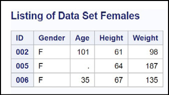
Suppose you have some raw data consisting of ID, gender, age, height, and weight. Earlier in this book, you developed a simple DATA step to read this collection of data. Suppose you want to create a SAS data set from the raw data, but you only want to see the female subjects. You have to use an IF statement because WHERE statements can only be used to subset SAS data sets. A demonstration of a subsetting IF is shown below.
Program 14.5: Demonstrating the Subsetting IF Statement
data Females;
   input @1  ID     $3.
         @4  Gender $1.
         @5   Age    3.
         @8  Height  2.
         @10 Weight  3.;
   if Gender = ‘F’;
datalines;
001M 5465220
002F10161 98
003M 1770201
004M 2569166
005F   64187
006F 3567135
;

title “Listing of Data Set Females”;
proc print data=Females;
   id ID;
run;
Notice that the IF statement does not have a THEN clause. This special IF statement, known as a subsetting IF, works like this: If the statement is true, the program continues; if the statement is false, the program returns to the top of the DATA step to read another line of data. Because an implicit output is performed at the bottom of the DATA step, only females will be in the resulting data set. Here is the listing.
Figure 14.7: Output from Program 14.5
A More Efficient Way to Subset Data When Reading Raw Data
Being a compulsive programmer, this author can’t leave this section without showing you a more efficient way to write Program 14.5. Why read all of the data for males when you are not going to keep it? It is better to read just the single byte of data for Gender and only if it is equal to ‘F’ read the remaining data. Here is the program—the explanation follows:
Program 14.6: Demonstrating a Trailing @
data Females;
   input @4  Gender $1. @;
   if Gender = ‘F’ then
      input @5   Age    3.
            @8  Height  2.
            @10 Weight  3.;
   else delete;
datalines;
001M 5465220
002F10161 98
003M 1770201
004M 2569166
005F   64187
006F 3567135
;
You might ask, “What is the @ sign doing at the end of the first INPUT statement?” Here’s the explanation: If you have more than one INPUT statement in a DATA step, SAS will go to the next line of data each time it encounters another INPUT statement. The @ sign at the end of the line is called a trailing @ and it tells SAS to “hold the line” and do not go to the next line of data when you encounter the next INPUT statement. Without the trailing @, the program would read the value of Gender from one line and input the other values from the next line.
The trailing @ on the first INPUT statement enables you to test the value of Gender and if it is equal to ‘F’ to read the values of Age, Height, and Weight from the same line of data. If Gender is not equal to ‘F’, the program executes the DELETE statement. This causes a return to the top of the DATA step without having to read the other values on the input record. Keep the trailing @ in mind whenever you need to read a portion of your data to decide how to read other values from the same line.
Creating Several Data Subsets in One DATA Step
If you need to create several subsets from a single SAS data set, you can reduce processing time by creating multiple SAS data sets in one DATA step. Doing this reduces processing time because you read through the data just once instead of multiple times. This is especially important when you are dealing with large files. For example, suppose you want to create three data sets from the SASHELP.Retail data set, each for a separate year. Here’s how to do it.
Program 14.7: Creating Several SAS Data Sets in One DATA Step
data Year1980 Year1981 Year1982;
   set SASHELP.Retail;
   if Year = 1980 then output Year1980;
   else if Year = 1981 then output Year1981;
   else if Year = 1982 then output Year1982;
run;
You name each of the data sets you want to create in the DATA statement. Next, you test the value of Year and use an OUTPUT statement, outputting observations to the appropriate data set. It is important to name the data set in the OUTPUT statement. If you use an OUTPUT statement without naming a data set, the program will output an observation to each of the data sets named in the DATA statement. One additional and important feature of this program is that when you include an OUTPUT statement in a DATA step, SAS does not perform an automatic output at the bottom of the DATA step.
When you run Program 14.7, the three data sets, Year1980, Year1981, and Year1982, are created.
Combining SAS Data Sets (Combining Rows)
One way to combine two or more data sets is to “stack them up” one on top of the other (also referred to as concatenation). For example, you might have data sets for each of the four quarters of the year and want to put them together to create a data set with all the data for the year. The simple example that follows shows how to do this using a SAS DATA step.
For this example, you have two data sets (cleverly called One and Two). They are shown below.
Figure 14.8: Data Sets One and Two
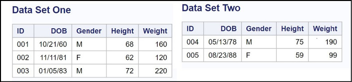
You use a SET statement to combine these two data sets, one after the other, like this:
Program 14.8: Using a SET Statement to Combine Two SAS Data Sets
data Both;
   set One Two;
run;
You list each of the data sets you want to combine in the SET statement. The program first reads all the observations from data set One. When it reaches the end of the file, it switches to data set Two and continues to read observations from data set Two until it reaches the end of that file. The result is all the observations from the two data sets.
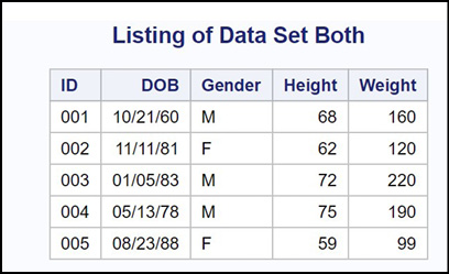
Here is a listing of data set Both.
Figure 14.9: Listing of Data Set Both
In case you want to run this program as is or with modifications, the program to create data sets One and Two is listed here.
Program 14.9: Program to Create Data Sets One and Two
data One;
   informat ID $3. DOB mmddyy10. Gender $1.;
   input ID DOB Gender Height Weight;
   format DOB mmddyy10.;
datalines;
001 10/21/1950 M 68 160
002 11/11/1981 F 62 120
003 1/5/1983 M 72 220
;

data Two;
   informat ID $3. DOB mmddyy10. Gender $1.;
   input ID DOB Gender Height Weight;
   format DOB mmddyy10.;
datalines;
004 5/13/1978 M 70 190
005 8/23/1988 F 59 98
;
Adding a Few Observations to a Large Data Set (PROC APPEND)
If your goal is to add observations (typically from a relatively small data set) to a large data set, you can, of course, use a SET statement and list the names of the two data sets, like this:
Program 14.10: Using a SET Statement to Solve the Problem
Data Both;
   Set Big Small;
run;
When you run this program, SAS will first read all the observations from data set Big and, when it reaches the end of the file, it will then read all the observations from data set Small.
If this is something that you need to do often, you might be concerned about efficiency, especially if data set Big is really big (millions or tens of millions of observations). A much more efficient method is to use PROC APPEND. A program that accomplishes the same goal as Program 14.10 (almost) is demonstrated in Program 14.11.
Program 14.11: Using PROC APPEND to Add Observations from One Data Set to Another
proc append base=Big Data=Small;
run;
You name the first data set in the BASE= procedure option and the data set to be added in the DATA= procedure option. This program does not need to read any observations from data set Big—it strips the end-of-file marker from the end of data set Big and then appends the new observations. If data set Big is large, this is a huge improvement in efficiency over using a SET statement. As with most things that look really quick and easy, there is a catch: In this program, you are replacing data set Big with the contents of Big and Small. If you have errors or bad data in data set Small, it is not easy to undo the process. It would be a good idea to have a backup copy of Big somewhere.
This method should only be used when you are confident that: One, the data that you are adding does not contain errors; and two, data set Small has all the same variables and attributes (especially character variable lengths) as data set Big. The reason for this is that the data descriptor (containing all the information such as variable types and lengths) is taken from data set Big.
If, for example, you had a character variable in data set Small that had a longer length than a variable of the same name in data set Big, that variable would be truncated. As a matter of fact, PROC APPEND would not even run in this situation unless you added an option called FORCE. The opinion of this author is that if you need to use the FORCE option, you had better know exactly what you are doing. One final point: If you have variables that have different names in the two data sets but are otherwise equivalent, you can use a RENAME= data set option to rename variables in one data set to match the variable names in the other data set.
If you have two or more data sets that are so large that, when put together, it would be difficult or impossible to sort the result, you can sort each of the data sets first and then interleave them. That is, you can add observations to the resulting data set from each of the constituent data sets so that the result is in sorted order. All that is necessary to accomplish this is to follow the SET statement with a BY statement, listing the variables that define the sorted order. Here is an example:
Program 14.12: Demonstrating How to Interleave Two or More Data Sets
*Note: data sets One, Two, and Three are sorted by ID;
data Combined;
   set One Two Three;
   by ID;
run;
The resulting data set (Combined) will be in ID order.
Merging Two Data Sets (Adding Columns)
By merging, we usually mean adding extra columns (variables) to a SAS data set based on one or more matching variables (such as ID or Name) from another data set. In SQL terms, you would be doing a join (inner, left, right, or, full). Imagine you are collecting clinical data on some patients. In one data set, you have ID, gender, and date of birth—in another data set, you have measurements such as weight, heart rate, and blood pressure. When it is time to analyze your data, you want to combine data from these two data sets. The program below creates two data sets, Patients and Visits.
Program 14.13: Creating the Patients and Visits Data Sets
data Patients;
   informat ID $4. Gender $1. DOB mmddyy10.;
   input ID Gender DOB;
   format DOB date9.;
datalines;
0001 M 10/10/1980
0023 F 1/2/1977
1243 M 6/17/2000
0002 M 8/23/1981
4535 F 2/25/1967
;

data Visits;
   informat ID $4. Visit_Date mmddyy10.;
   input ID Visit_Date Weight HR SBP DBP;
   format Visit_Date date9.;
datalines;
0023 2/10/2015 122 76 122 78
4535 10/21/2014 155 78 138 88
0001 11/11/2014 210 68 118 78
;
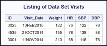
A listing of these two data sets is shown next:
Figure 14.10: Listing of Data Sets Patients and Visits

In order to combine (merge) these two data sets, you must first sort each of them by the variable (or variables) that you plan to use to match the two data sets. Here is the program, followed by an explanation:
Program 14.14: Merging Two SAS Data Sets
proc sort data=Patients;
by ID;
run;
proc sort data=Visits;
by ID;
run;
data Merged;
merge Patients Visits;
by ID;
run;
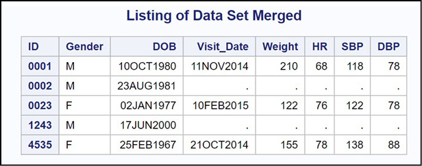
title “Listing of Data Set MERGED”;
proc print data=Merged;
id ID;
run;
You use PROC SORT to sort both data sets by ID. Next, you use a MERGE statement to combine the patient and visit data and a BY statement to instruct the program to use ID as the matching variable. Here is the resulting data set.
Figure 14.11: Output from Program 14.4
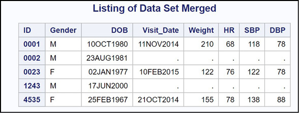
What you see here is all the observations from the Patients data set matched with all the observations in the Visits data set (known as a full join in SQL), even if there is no corresponding visit for a particular ID.
This is probably not what you want. In this example, you most likely want to see a listing of only those patients who were in the Visits data set. Luckily, SAS has a way to control which observations will be included in the merged data set. Enter the IN= data set option.
Controlling Which Observations Are Included in a Merge (IN= Data Set Option)
You have previously seen a WHERE= data set option. You can now add to your collection of data set options by learning about the IN= data set option. Here’s how it works:
When you are merging two data sets, you might find a matching ID in both data sets or you might only find an ID in one but not the other data set. To determine whether a data set is making a contribution on a particular merge, you add an IN= variable_name data set option following each of the two data sets in the MERGE statement. Let’s examine the value of these variables (called contributor variables by some SAS programmers) in the following program.
Program 14.15: Demonstrating the IN= Data Set Option
*Note: both data set previously sorted by ID;
data Merged;
   merge Patients(in=In_Patients) Visits(In=In_Visits);
   by ID;
   put ID= In_Patients= In_Visits=;
run;
The variable name following the IN= data set option can be any valid SAS name. However, this author likes to use names that help you remember which variable goes with which data set. Hence, the names In_Patients and In_Visits.
These two variables are temporary variables. That is, they are not included in the output data set. They are available only during the DATA step to help you determine how to perform the merge. A PUT statement was added to Program 14.15 so that you can examine these two variables. Here is the relevant section of the SAS log:
Figure 14.12: Partial Listing of the SAS Log from Program 14.15
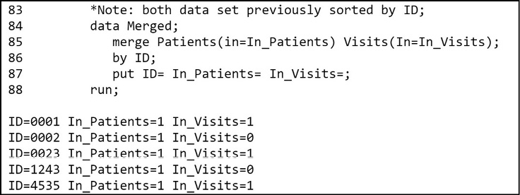
In each observation, the IN= variable is a 1 when that data set is contributing to the merge and 0 otherwise. Patient 0001 is in both data sets, so the value of the two IN= variables is 1. Patient 0002 is in the Patients data set but not the Visits data set, so In_Patients is a 1 and In_Visits is a 0 for this observation.
You can use the IN= variables to control which observations you want to include in the output data set. For example, to include only observations where there is a contribution from both data sets (referred to as an inner join is SQL), you would use:
if In_Patients=1 and In_Visits=1;
This can also be written as:
if In_Patients and In_Visits;
You do not need to include the equals 1 because SAS understands that these variables are either 1 or 0 (interpreted as true or false).
In this example, every patient in the Visits data set was matched to a record in the Patients data set. In the real world, this would not always be the case. The next program creates a data set containing patients in the Visits data set who are matched with the data in the Patients data set.
To make the program more general, statements were added to print an error message for any patient in the Visits data set who is missing from the Patients data set. It is good programming to expect the unexpected! Here is the program.
Program 14.16: Using the IN= Data Set Option to Control the Merge Operation
*Note: Both data sets already sorted by ID;
title “Listing of Patients with Visits Who are Not in the Patients Data Set”;
data Only_Visit_Patients;
file print;
merge Patients(in=In_Patients) Visits(in=In_visits);
by ID;
if In_Visits then output;
if In_Visits and not In_Patients then
put “Patient “ ID “not found in the Patients data set.”;
run;
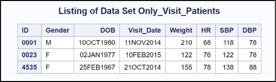
title “Listing of Data Set Only_Visit_Patients”;
proc print data=Only_Visit_Patients;
id ID;
run;
You test the value of the variable In_Visits, and only output observations where In_Visits is true. If there is an ID in the Visits data set that does not have an observation in the Patients data set, a message is written. By default, PUT statements write data to the SAS log. By including the statement FILE PRINT, the output from this PUT statement will be sent to the RESULTS window. It turns out that there were no patients who were in the Visits data set and not in the Patients data set, so no messages were printed by the PUT statement. Here is the output.
Figure 14.13: Output from Program 14.16
Performing a One-to-Many or Many-to-One Merge
If you want to merge two data sets where one data set has more than one observation for your choice of BY variable(s) and the other data set has exactly one observation for the same BY variable(s), you can still perform a merge. For this example, you want to merge patient data (ID, Gender, and DOB) with visit data (ID, date of visit, HR, SBP, and DBP). To demonstrate this merge, we will use the Patients data set (see Program 14.13) and a new data set, Many_Visits, which contains several visits for each patient. The program to create the Many_Visits data set is shown in Program 14.17.
Program 14.17: Creating Another Data Set to Demonstrate a One-to-Many Merge
data Many_Visits;
   informat ID $4. Visit_Date mmddyy10.;
   input ID Visit_Date HR SBP DBP;
   format Visit_Date date9.;
;
datalines;
0023 2/10/2015 122 76 122 78
0023 3/10/2015 120 74 120 76
4535 10/21/2014 155 78 138 88
0001 11/11/2014 210 68 118 78
0001 12/20/2014 210 68 120 82
0001 1/5/2015 212 70 210 80
;
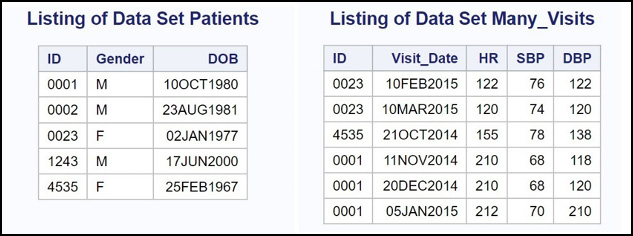
For reference, both data sets (Patients and Many_Visits) are displayed below.
Figure 14.14: Listing of Data Sets Patients and Many_Visits
You can now sort and merge the two data sets like this.
Program 14.18: Performing a One-to-Many Merge
proc sort data=Patients;
   by ID;
run;

proc sort data=Many_Visits;
   by ID;
run;

data One_to_Many;
   merge Patients Many_Visits;
   by ID;
run;

title “Listing of data set One_To_Many”;
proc print data=One_to_Many;
   id ID;
run;
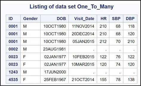
When you run this program, the variables Gender and DOB from the Patients data set are combined with matching observations from the Many_Visits data set (based on ID) to create the data set One_To_Many, as shown in the listing below.
Figure 14.15: Output from Program 14.18
In this example, you could reverse the order of the two data sets (performing a many-to-one merge) and the result would be identical to the one obtained here.
CAUTION: Do not attempt to merge two data sets where there are multiple observations for each BY variable in both data sets and the number of multiples is not the same in both files.
Merging Two Data Sets with Different BY Variable Names
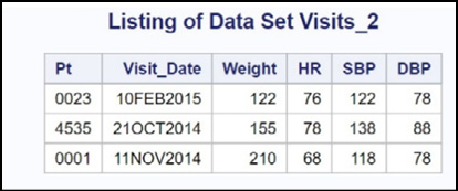
You might find yourself needing to merge two data sets, but the BY variable has a different variable name in each of the two files (this is corollary number 17 of Murphy’s Law). The solution to this problem is actually very simple. Let’s redo Program 14.14, but make a slight change to the data set Visits. The new data set (Visits_2) has all the same values of data set Visits except that the ID variable is named Pt.
Here is a listing of data set Visits_2:
Figure 14.16: Listing of Data Set Visits_2
Before we continue, here is the program that was used to create the data set Visits_2 (in case you want to try this yourself):
Program 14.19: Program to Create Data Set Visits_2
data Visits_2;
   informat Pt $4. Visit_Date mmddyy10.;
   input Pt Visit_Date Weight HR SBP DBP;
   format Visit_Date date9.;
datalines;
0023 2/10/2015 122 76 122 78
4535 10/21/2014 155 78 138 88
0001 11/11/2014 210 68 118 78
;
In order to merge the two files Patients and Visits_2, you have to rename one of the variables (either ID or Pt) so that both BY variables have the same name. You do this with a RENAME= data set option. In this example, you are going to rename the variable Pt in the Visits_2 data set to ID.
Program 14.20: Using a RENAME= Data Set Option to Rename the Variable Pt to ID
proc sort data=Patients;
   by ID;
run;

proc sort data=Visits_2;
   by Pt;
run;

data Merged;
   merge Patients
         Visits_2(rename=(Pt = ID));
by ID;
run;

title “Listing of Data Set Merged”;
proc print data=Merged;
   id ID;
run;
This is another opportunity to get confused with the parentheses. Remember, the outer-most set holds all of the data set options, and the inner-most set is a list of old variable names and new variable names. The form of the RENAME= data set option is:
Data-Set-Name(rename=(Old-name1=New_Name1 Old_Name2=New_Name2 . . .));
You can rename as many variables as needed using the RENAME= data set option. However, the two variables on each side of the equal sign must be the same type (either character or numeric).
Here is the output from Program 14.20.
Figure 4.17: Output from Program 14.20
If you have a situation where the two variables that you would like to use in a merge are not the same type, you have to do a bit more work. The solution to this problem is discussed in the next section.
Merging Two Data Sets with One Character and One Numeric BY Variable
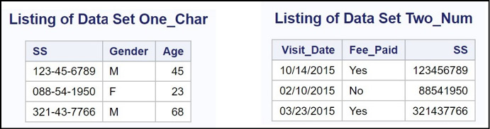
Because you cannot use a RENAME= data set option with two variables of different types, you need to create a new variable with the same name and type as the matching variable in the other data set. In this example, you have a variable called SS (Social Security number) in both files; however, one is stored as a character string and the other as a numeric value. Here is a listing of the two data sets you want to merge.
Figure 14.18: Listings of Data Set One_Char and Two_Num
The program to create these two data sets is listed next, in case you want to try it out for yourself.
Program 14.21: Program to Create Data Sets One_Char and Two_Num
data One_Char;
   informat SS $11. Gender $1.;
   input SS Gender Age;
datalines;
123-45-6789 M 45
088-54-1950 F 23
321-43-7766 M 68
;
data Two_Num;
   informat Visit_Date mmddyy10. Fee_Paid $3.;
   input SS Visit_Date Fee_Paid;
   format Visit_Date mmddyy10.;
datalines;
123456789 10/14/2015 Yes
088541950 2/10/2015 No
321437766 3/23/2015 Yes
;
Before you conduct a merge, it is a good idea to run PROC CONTENTS (or examine the variables using SAS Studio) to ensure that the BY variables are the same type (and length). With this in mind, here is a section of PROC CONTENTS output for each of the two data sets.
Figure 14.19: Output from PROC CONTENTS for Data Set One_Char
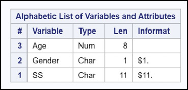
Figure 14.20: Output from PROC CONTENTS for Data Set Two_Num
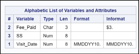
You can see that the variable SS is stored as character in data set One_Char and numeric in data set Two_Num.
It’s time to merge these two data sets. You have a choice—convert the character variable to a numeric variable or vice versa. Let’s choose the latter—changing the numeric variable to character. Here is the program.
Program 14.22: Merging Two Data Sets with One Character and One Numeric BY Variable
data Two_Char;
   set Two_Num(rename=(SS = SS_Num));
   SS = put(SS_Num,SSN11.);
   drop SS_Num;
run;

proc sort data=One_Char;
   by SS;
run;

proc sort data=Two_Char;
   by SS;
run;

Data One_and_Two;
   merge One_Char Two_Char;
   by SS;
run;

title “Listing of Data Set One_and_Two”;
proc print data=One_and_Two noobs;
run;
There is quite a lot going on here. To start, you need to create a new data set (called Two_Char in this example) with a variable called SS that is stored as a character value. You use a SET statement to read the observations from data set Two_Num. Because you need the final character variable to be called SS, you use the RENAME= data set option to rename the original, numeric variable SS to SS_Num.
The next step is to use the PUT function to perform a numeric-to-character conversion. Here’s how it works: There is a SAS format called SSN11. that writes out numeric representations of Social Security numbers as 11-byte character strings, complete with leading zeros and hyphens. The PUT function takes two arguments. The first argument is the variable that you want to convert (SS_Num in this example), and the second argument is a format that you want to use to format this value. The result is a character string in the same form as in data set One_Char. Because you no longer need (or want) the variable SS_Num in your data set, you use a DROP statement. This statement says that when SAS writes out observations to a data set, it should not include any variables listed in the DROP statement.
Output from Program 14.22 is listed next:
Figure 14.21: Output from Program 14.22
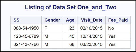
That wasn’t easy, but it is very likely that some time in your programming career, you will face this problem. Now you know the solution.
Updating a Master File from a Transaction File (UPDATE Statement)
The final (yeah!) section of this chapter describes how to update values in a master file, using transaction data in a transaction file. In this example, you have a file of item numbers, descriptions, and prices, and you want to modify the file to change the price of a few items. Here is a program to create the master Price file and a listing of the file.
Program 14.23: Program to Create the Master File
data Price;
   input @1  Item_Number $5.
         @7  Description $10.
         @18 Price;
datalines;
12345 Hammer     11.98
22222 Saw        25.89
44010 Nails 10p  17.95
44008 Nails 8p   15.56
;

title “Listing of Data Set Price”;
proc print data=Price;
   id Item_Number;
run;
Here is the listing:
Figure 14.22: Data Set Price

You want to change the price of the hammer (item number 12345) to $12.98 and the price of 8 penny nails (item 44008) to $16.50. You first create a data set with these two items (you only need the item number and the new price). This will be your transaction data set.
Program 14.24: Creating the Transaction Data Set
data Transact;
   informat Item_Number $5.;
   input Item_Number Price;
datalines;
12345 12.98
44008 16.50
;

title “Listing of Data Set Transact”;
proc print data=Transact;
   id Item_Number;
run;
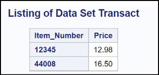
This is the listing:
Figure 14.23: Output from Program 14.24
Here is the program to update the prices in your master file:
Program 14.25: Updating Your Master File Using a Transaction Data Set
proc sort data=Price;
   by Item_Number;
run;

proc sort data=Transact;
   by Item_Number;
run;

data Price_10Oct2020;
   update Price Transact;
   by Item_Number;
run;

title “Listing of Data Set Price_10Oct2020”;
proc print data= Price_10Oct2020;
   id Item_Number;
run;
You first sort both data sets by Item_Number. Next, you decide to give the new Price data set a different name—Price10Oct2020. Giving the new Price data set a new name is a good idea as it helps prevent confusion. Finally, you use an UPDATE statement to update the prices in the original Price data set. UPDATE is similar to MERGE. However, in a MERGE, if you have a variable in the second data set with the same name as a variable in the first data set, the value in the second data set will replace the value in the first data set, even if that value is a missing value. When you use the UPDATE statement, a missing value in the second data set does not replace the value in the first data set—just what you want to happen. Here is the listing:
Figure 14.24: Output from Program 14.25
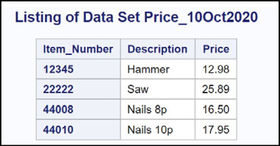
You see that the two prices are updated. Keep the UPDATE statement in mind whenever you need to replace values in one data set using values from another data set. It is one of the often-forgotten SAS statements.
This was clearly one of the more difficult chapters. However, many, if not most, programming problems require you to manipulate data from multiple data sets. If you know and love SQL, you can use that knowledge to combine your SAS data sets. The choice of SET, MERGE, and UPDATE versus SQL is not always easy. We often use what we know best. Because PROC SQL came much later in the evolution of SAS, many of the “older” SAS programmers choose to use DATA step processing.
1. Starting with the SASHELP data set Fish, create a data set called Small_Perch that contains only perch that weigh less than 50 (whatever the weigh units are). Do this using a WHERE statement.
2. Repeat Problem 1 using a WHERE= data set option.
3. Run the program shown below. If you don’t want to enter it, you will find this program included in a program called “Programs for Data Sets.sas”, included in your download of data for this book. Use a subsetting IF statement to include only those subjects where the sum of Q1–Q3 is greater than using equal to 6.
Program for Problem Sets 1
data Questionnaire;
informat Gender 1. Q1-Q4 $1. Visit date9.;
input Gender Q1-Q4 Visit Age;
format Visit date9.;
datalines;
1 3 4 1 2 29May2015 16
1 5 5 4 3 01Sep2015 25
2 2 2 1 3 04Jul2014 45
2 3 3 3 4 07Feb2015 65
;
4. Starting with the SASHELP data set Cars, create two temporary data sets. The first one (Cheap) should include all the observations from Cars where the MSRP (manufacturer’s suggested retail price) is less than or equal to $11,000. The other (Expensive) should include all the observations from Cars where the MSRP is greater than or equal to $100,000. Use a KEEP= data set option to include only the variables Model, Type, Origin, and MSRP from the Cars data set. Create these two data sets in one DATA step. Use PROC PRINT to list the observations in Cheap and Expensive. Even though there are no missing values for the variable MSRP, write your program so that any observation with a missing value for MSRP will not be written to data set Cheap.
5. Run Program for Problem Sets 6 to create two data sets (FirstQtr and SecondQtr). Then create a new data set (FirstHalf) that contains all the observations from FirstQtr and SecondQtr.
data FirstQtr;
input Name $ Quantity Cost;
datalines;
Fred 100 3000
Jane 90 4000
April 120 5000
;
data SecondQtr;
input Name $ Quantity Cost;
datalines;
Ron 200 9000
Jan 210 9500
Steve 177 5400
;
6. Repeat Problem 5, except use PROC APPEND to combine the observations from data sets FirstQtr and SecondQtr. Because you want the resulting data set to be called FirstHalf, you will first need to make a copy of FirstQtr that is called First_Half.
7. Run Program for Problem Sets 7. Then create a new data set (Both) that contains ID, X, Y, Z, and Name. Include only those IDs that are in both data sets.
data First;
input ID $ X Y Z;
datalines;
001 1 2 3
004 3 4 5
002 5 7 8
006 8 9 6
;
data Second;
input ID $ Nane $;
datalines;
002 Jim
003 Fred
001 Susan
004 Jane
;
8. Repeat Problem 7, except include all observations from each data set, even if there is no corresponding ID in one of the files.
9. Run Program for Problem Sets 8. Write a program to create a new data set called New_Prices, where the price of item X200 is $410 and the price of item A123 is $121. Caution: Item _Number is a character variable and the data set is not sorted by Item_Number.
data Prices;
input Item_Number $ Price;
datalines;
A123 $123
B76 4.56
X200 400
D88 39.75
;