Chapter 15: Describing SAS Functions
You have already seen a number of SAS functions in earlier chapters of this book. This chapter explores some of the most useful SAS functions that work with numeric and character data.
To review, SAS functions either return some system value or perform some calculation and return a value. Here are some useful facts about SAS functions:
● All SAS function names are followed by zero or more arguments, placed in parentheses following the function name.
● Although there are some exceptions, arguments to SAS functions can be variable names (the most common type of argument), constants (numbers for numeric functions, character values in quotation marks for character arguments), expressions (such as arithmetic expressions), or even other functions.
● Functions can only return a single value and, in most cases, the arguments to SAS functions do not change after you execute the function.
You will also see two CALL routines in this chapter. CALL routines are something like functions except for two important differences: One, some or all of the arguments can change value after the call; and two, you do not use a CALL routine in an assignment statement.
The following examples, using the WEEKDAY function (which returns the day of the week given a SAS date), demonstrate the variety of arguments that are valid with most SAS functions:
● Day = weekday(Date) where Date is the name of a SAS variable
● Day = weekday(20013) a numeric constant
● Day = weekday(‘01Jan2015’d) a date constant
● Day = weekday(today()) where Today is a SAS function that returns the current date
● Day = weekday(Date + 1) an arithmetic expression giving the day of the week one day after Date
Describing Some Useful Numeric Functions
Each function in this chapter will be described and you will see either a full program or a statement showing how the function works.
What it does: The MISSING function returns a value of true (1) if the argument is a missing value and false (0) otherwise.
Arguments: A character or numeric value
Examples:
Program 15.1: Demonstrating the MISSING Function
data Old_Miss;
   input ID $ Age;
   if missing(Age)      then Age_group = .;
      else if Age le 50 then Age_group = 1;
      else                   Age_group = 2;
datalines;
001 15
002 .
003 78
004 26
;

title “Listing of Data Set Old_Miss”;
proc print data=Old_Miss noobs;
run;
Explanation: You use the MISSING function to test if Age is a missing value. If so, you assign a missing value to the variable Age_Group. Here is the listing from Program 15.1:
Figure 15.1: Output from Program 15.1
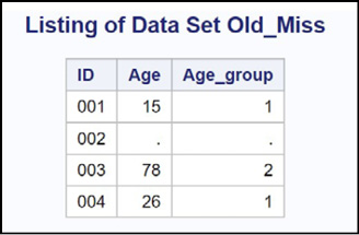
Notice that Age_Group has a missing value for ID 002.
What it does: Returns the number of nonmissing values in the list of arguments
Arguments: One or more numeric values. If any of the arguments are in the form Variable1-VariableN, the list must be preceded by the keyword OF.
Examples:
X1=1; X2=.; X3=3; Age=27; Wt=.; Ht=68;
n(of X1-X3) = 2
n(Age, Wt, Ht) = 2
Explanation:
In the list of variables X1–X3, there are two nonmissing values.
Among the three variables Age, Wt, and Ht, there are two nonmissing values.
What it does: Returns the number of missing values in the list of arguments
Arguments: One or more numeric values. If any of the arguments are in the form Variable1-VariableN, the list must be preceded by the keyword OF.
Examples:
X1=1; X2=.; X3=3; Age=27; Wt=.; Ht=68;
nmiss(of X1-X3) = 1
nmiss(Age, Wt, Ht) = 1
Explanation:
In the list of variables X1–X3, there is one missing value.
Among the three variables Age, Ht, and Wt, there is one missing value.
What it does: Returns the sum of the arguments. In performing this operation, missing values are ignored. If all the arguments are missing, the result is a missing value.
Arguments: One or more numeric values. If any of the arguments are in the form Variable1-VariableN, the list must be preceded by the keyword OF.
Examples:
X1=1; X2=.; X3=3; Age=27; Wt=.; Ht=68;
sum(of X1-X3) = 4
sum(Age, Wt, Ht) = 95
Explanation:
Because X2 is a missing value, the result is the sum of 1 and 3.
The sum of Age (27) and Ht (68) is 95. The missing value is ignored.
Because the SUM function returns a missing value when all of its arguments are missing values, a popular trick to return a value of 0 in this situation is to include a 0 as one of the arguments. For example,
If Cost1–Cost5 are all missing, the expression
sum(0,of Cost1-Cost5)
will return a value of 0.
What it does: Returns the mean (average) of the arguments. In performing this operation, missing values are ignored. If all the arguments are missing, the result is a missing value.
Arguments: One or more numeric values. If any of the arguments are in the form Variable1-VariableN, the list must be preceded by the keyword OF.
Examples:
X1=1; X2=.; X3=3; Age=27; Wt=.; Ht=68;
mean(of X1-X3) = 2
mean(Age, Wt, Ht) = 47.5
Explanation:
X2 is a missing value and is ignored. The mean is computed as (1 + 3) / 2.
The mean of Age (27) and Ht (68) is 47.5. The missing value is ignored.
What it does: Returns the smallest nonmissing value of its arguments. If all the arguments are missing, the result is a missing value.
Arguments: One or more numeric values. If any of the arguments are in the form Variable1-VariableN, the list must be preceded by the keyword OF.
Examples:
X1=1; X2=.; X3=3; Age=27; Wt=.; Ht=68;
min(of X1-X3) = 1
min(Age, Wt, Ht) = 27
Explanation:
1 is the smallest nonmissing value of the arguments.
27 is the smallest nonmissing value.
What it does: Returns the largest nonmissing value of its arguments. If all the arguments are missing, the result is a missing value.
Arguments: One or more numeric values. If any of the arguments are in the form Variable1-VariableN, the list must be preceded by the keyword OF.
Examples:
X1=1; X2=.; X3=3; Age=27; Wt=.; Ht=68;
max(of X1-X3) = 3
max(Age, Wt, Ht) = 68
Explanation:
3 is the largest value of the arguments.
The largest value is 68.
What it does: Returns the nth smallest nonmissing value of its arguments. If there is no nth nonmissing value, the function returns a missing value.
Arguments: If the first argument is a 1, the function returns the smallest (nonmissing) value in the list of numeric values; if it is a 2, the function returns the second smallest value; and so on. The second to last arguments are numeric values. If any of the arguments are in the form Variable1-VariableN, the list must be preceded by the keyword OF.
Examples:
X1= 1; X2=.; X3=3; X4=2;
smallest(1,of X1-X4) = 1
smallest(2,of X1-X4) = 2
smallest(3,of X1-X4) = 3
smallest(4,of X1-X4) = . (missing value)
Explanation:
When the first argument is equal to 1, the result is identical to the MIN function.
When it is equal to 2, it returns the second (nonmissing) smallest number.
The third nonmissing smallest value is 3.
When you are asking for the fourth smallest number, the function returns a missing value because there is no fourth smallest number.
What it does: Returns the nth largest nonmissing value of its arguments. If there is no nth nonmissing value, the function returns a missing value.
Arguments: If the first argument is a 1, the function returns the largest (nonmissing) value in the list of numeric values; if it is a 2, the function returns the second largest value; and so on. The second through last arguments are numeric values. If any of the arguments are in the form Variable1-VariableN, the list must be preceded by the keyword OF.
Examples:
X1= 1; X2=.; X3=3; X4=2;
largest(1,of X1-X4) = 3
largest(2,of X1-X4) = 2
largest(3,of X1-X4) = 1
largest(4,of X1-X4) = . (missing value)
Explanation:
When the first argument is equal to 1, the result is identical to the MAX function.
When it is equal to 2, it returns the second (nonmissing) largest number.
The third largest number is 1.
When you are asking for the fourth largest number, the function returns a missing value because there is no fourth largest number.
Programming Example Using the N, NMISS, MAX, LARGEST, and MEAN Functions
The program that follows demonstrates how several of the functions just described can work in concert to produce a very useful result. Here is the problem:
You are given the results of a psychological study. There are 10 variables, Q1 to Q10. You are asked to compute several scores as follows:
1. Score1: the mean of the first five questions (Q1–Q5). Compute this value only if there are three or more nonmissing values.
2. Score2: the mean of Q6–Q10. Compute this mean if there are two or fewer missing values.
3. Score3: the highest score of Q1–Q10.
4. Score4: the sum of the three highest scores of Q1–Q10.
Program 15.2: Program Demonstrating Several Functions (N, NMISS, MAX, LARGEST, and MEAN)
data Score;
   input ID $ Q1-Q10;
   if n(of Q1-Q5) ge 3 then Score1 = mean(of Q1-Q5);
   if nmiss(of Q6-Q10) le 2 then Score2 = mean(of Q6-Q10);
   Score3 = max(of Q1-Q10);
   Score4 = sum(largest(1,of Q1-Q10),
                largest(2,of Q1-Q10),
                largest(3,of Q1-Q10));
datalines;
001 9 7 8 6 7 6 . . 9 2
002 . . . . 9 8 7 8 9 9
003 6 7 6 7 6 . . . 9 9
;
title “Listing of Data Set Score”;
proc print data=Score noobs;
run;
Explanation: The combination of N and MEAN or NMISS and MEAN is very useful for solving problems of this nature. Also, determining the second or third largest value in a list of values is very difficult without using the LARGEST function. Here is the output.
Figure 15.2: Output from Program 15.2
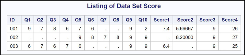
There are missing values for Score1 and Score2 because the criteria for computing a score were not met.
What it does: Takes the first argument (character value) and “reads” it as if it were being read from text data in a file using an INFORMAT that you supply as the second argument of the function. The most popular use of this function is to perform character-to-numeric conversion.
Arguments: The first argument is a character value (typically a character variable). The second argument is the informat that you want to use to associate with the first argument.
Examples:
C_Num = ‘123’; C_Date = ‘10/21/1950’; C_Money = ‘$12,345.54’;
Num = input(C_num,12.); Num is the number 123
Date = input(C_Date,mmddyy10.); Date is a SAS date
Money = input(C_Money,Dollar12.); Money is a numeric variable
Explanation: In the first example, notice that the informat (12.) is much larger than you need (you only needed 3.). However, unlike reading data from a text file, the INPUT function will not read past the end of a character value, so there is no harm in choosing a large number for the numeric informat.
The second example shows how to convert a date, stored as a character string, into a true SAS date.
The last example uses the Dollar12. informat that strips dollar signs and commas from a value. Note that the Comma. informat also works for this example.
What it does: After the CALL statement executes, the values of all of the calling arguments are in ascending order. That is, this CALL routine can sort within an observation.
Arguments: One or more numeric variables. If any of the arguments are in the form Variable1-VariableN, the list must be preceded by the keyword OF.
Examples:
X1=7; X2=3; X3=9; X4=.; X5=2;
call sortn(of X1-X5);
The values of X1 to X5 are now:
X1=. X2=2 X3=3 X4=7 X5=9
call sortn(of X5 – X1);
The values of X1 to X5 are now:
X1=9 X2=7 X3=3 X4=2 x5=.
If you enter the arguments in reverse order, you can perform a descending sort of the values.
As a practical example, you have 10 test scores (Score1 to Score10) for each student (Stud_ID). You want to compute the mean of the eight highest scores.
Program 15.3: Using CALL SORTN to Compute the Mean of the Eight Highest Scores
data Test;
   input Stud_ID $ Score1-Score10;
   call sortn(of Score1-Score10);
   Mean_Top_8 = mean(of Score3-Score10);
datalines;
001 90 90 80 78 100 95 90 92 88 82
002 50 55 60 65 70 75 80 85 90 95
;
title “Listing of Data Set TEST”;
proc print data=Test;
   id Stud_ID;
   var Score1-Score10 Mean_Top_8;
run;
Here is the listing from Program 15.3.
Figure 15.3: Output from Program 15.3
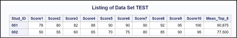
Explanation: Notice that the Score variables are now in ascending order. If you prefer, you can reverse the order of the arguments in the CALL SORTN routine and then compute the mean as mean(of Score1-Score8).
What it does: If you execute the LAG function for every iteration of the DATA step, it returns the value of its argument from the previous observation.
The true definition of the LAG function is that it returns the value of its argument the last time the function executed.
Arguments: A character or numeric variable
Examples:
Because SAS processes one observation at a time, you need special tools to be able to retrieve a value from an earlier observation. The LAG function is one of those tools. For this first example, you have daily stock prices, and you want to compare the current day’s price with that of the previous day. Here is the program.
Program 15.4: Demonstrating the LAG Function
data Stocks;
   informat Date mmddyy10.;
   input Date Price;
   Up_Down = Price - lag(Price);
   format Date mmddyy10.;
datalines;
1/1/2015 100
1/2/2015 98
1/3/2015 96
1/4/2015 101
1/5/2015 101
1/6/2015 104
;

title “Listing of Data Set Stocks”;
proc print data=Stocks noobs;
run;
Explanation: Because this program is executing the LAG function for every iteration of the DATA step, the variable Up_Down will be the current day’s price minus the price from the previous day. Here is the listing.
Figure 15.4: Output from Program 15.4
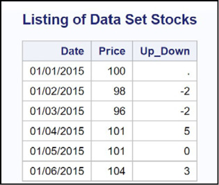
The value of Up_Down is missing in the first observation because that was the first time the LAG function executed and there was no previous value.
There is actually a whole family of LAG functions (LAG, LAG2, LAG3, etc.). LAG2 returns the value of its argument from two previous executions of the function, LAG3 three times, and so on. For example, you can use the Stocks data set to compute a three-day moving average as follows.
Program 15.5: Using the Family of LAGn Functions to Compute a Moving Average
data Moving;
   set Stocks;
   Yesterday = lag(Price);
   Two_Days_Ago = lag2(Price);
   Moving = mean(Price, Yesterday, Two_Days_Ago);
run;

title “Listing of Data Set Moving”;
proc print data=Moving noobs;
run;
Here is the output.
Figure 15.5: Output from Program 15.5
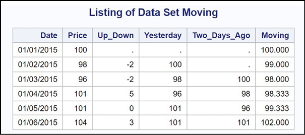
Explanation: The variable Moving represents a three-day moving average. You can decide not to output this value until you reach day three—your choice.
What it does: The value of DIF(X) is equal to X – LAG(X). Because one of the most common uses of the LAG function is to compute inter-observation differences, SAS created the DIF function to save you a few keystrokes when you write your programs.
Arguments: A numeric variable
Examples:
You can substitute the line:
Up_Down = dif(Price);
for the line that computes the difference of the current day price and the price from the day before in Program 15.4.
Describing Some Useful Character Functions
The functions discussed in this section all deal with character values. Because there are so many useful character functions, you will see them grouped into logical categories, such as functions that extract substrings, functions that combine strings, and functions that take strings apart.
Function Names: LENGTHN and LENGTHC
What it does: LENGTHN returns the length of a character value, not counting trailing blanks (blanks to the right of the string). If the argument is a missing value, the function returns a 0. LENGTHC returns the storage length of a character variable.
Arguments: A character value or a character variable
Examples:
Program 15.6: Demonstrating the Two Functions LENGTHN and LENGTHC
data How_Long;
   length String $ 5 Miss $ 4;
   String = ‘Abe’;
   Miss = ‘ ‘;
   Length_String = lengthn(String);
   Store_String = lengthc(String);
   Display = ‘:’ || String || ‘:’;
   Length_Miss = lengthn(Miss);
   Store_Miss = lengthc(Miss);
run;

title “Listing of Data Set HOW_LONG”;
proc print data=How_Long noobs;
run;
Explanation: This program demonstrates how the two functions LENGTHN and LENGTHC work. Looking at the output (below) should help clarify the difference between these two functions. The variable Display uses the concatenation operator (||) to place a colon on each side of String. This enables you to see any leading or trailing blanks in the value. Here is the output.
Figure 15.6: Output from Program 15.6
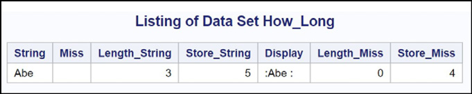
The variable String is assigned a length of 5, using a LENGTH statement. The LENGTHN function returns a 3, the length of String with the (2) trailing blanks not counted. The storage length, returned by the LENGTHC function, correctly shows that String has a length of 5. The variable Display is a colon, followed by ‘Abe’, followed by two blanks, followed by a colon.
Character missing values are represented by blanks. The number of blanks is equal to the storage length for that variable. However, when you are either assigning a missing value to a variable (as shown in the assignment statement for Miss) or testing if a character value is missing, you use a single blank in single or double quotation marks (you can also test for, or assign a missing value by using two quotation marks together, with no space—but a single blank is the standard). The LENGTHN function returns a length of 0 for the variable Miss while LENGTHC returns the storage length (4).
For nonmissing character values, an older function called LENGTH is identical to the newer LENGTHN function. However, if the argument is a missing value, the older LENGTH function returns a 1 instead of a 0. The LENGTHN function was introduced with SAS version 9, the same version where strings of zero length were allowed. By the way, the ‘N’ in the function name LENGTHN stands for null string.
Function Names: TRIMN and STRIP
What it does: TRIMN removes trailing blanks and STRIP removes both leading and trailing blanks. Note that the TRIMN function replaces the older TRIM function. The difference is that the TRIMN function returns a null string (a string of zero length) if its argument is a missing value, and the TRIM function returns a single blank when its argument is a missing value.
Both of these functions are particularly useful when you have character values that might contain leading or trailing blanks. Other functions that search strings for values such as digits or letters (see the ANY and NOT functions later in this chapter) search every position of a character value, including leading or trailing blanks. You usually want to remove leading and trailing blanks before using these searching functions.
Arguments: A character value
Examples:
Trail=’ABC ‘; Lead= ‘ ABC’; Both=’ ABC ‘;
|
Expression |
Value |
‘:’ || Trail || ‘:’ |
:ABC : |
‘:’ || trimn(Trail) || |
:ABC: |
‘:’ || Lead || ‘:’ |
: ABC: |
‘:’ || strip(Lead) || ‘:’ |
:ABC: |
‘:’ || trimn(Both) || ‘:’ |
: ABC: |
‘:’ || strip(Both) || ‘:’ |
:ABC: |
Explanation: The first example uses the concatenation operator to place a colon on each side of the variable Trail. Therefore, there are blanks between the ‘C’ and the colon.
In the second example, you use the TRIMN function to remove the trailing blanks before concatenating the final colon. Therefore, there are no blanks between the ‘C’ and the colon.
The third example concatenates a colon on each side of the variable Lead. Therefore, there are blanks between the first colon and the ‘A’.
In the fourth example, the STRIP function removes leading and trailing blanks from the argument. Therefore, there are no blanks between the colons and ‘ABC’.
In the fifth example, the TRIMN function removes the trailing blanks from Both so that there are blanks between the first colon and the ‘A’ and no blanks between the ‘C’ and the final colon.
The last example uses the STRIP function to remove leading and trailing blanks from Both, resulting in no blanks between the first colon and the ‘A’ or the ‘C’ and the final colon.
It is unusual for a SAS character value to contain leading blanks because the $W. informat left-justifies character values. However, if you are not sure if a variable contains leading blanks, use the STRIP function instead of the TRIMN function, just to be sure.
Before we leave these two functions, let’s take a look at the following statements:
String = ‘ABC ‘;
String = trimn(String);
What is the value of String? The answer is ‘ABC ‘. The reason is that although the TRIMN function removed the trailing blanks, when you then assign the trimmed value to a string of length 6, the trailing blanks return.
Function Names: UPCASE, LOWCASE, and PROPCASE (Functions That Change Case)
What it does: The three functions in this group all change the case of their argument. This is especially useful when you have character data that is entered in different cases (some upper, some lower, some mixed).
Arguments: LOWCASE and UPCASE: A character value. PROPCASE: A character value and, optionally, a second argument where you list your choice of delimiters.
You can probably guess the purpose of the first two functions, UPCASE and LOWCASE. UPCASE converts all letters in its argument to uppercase, and LOWCASE converts letters to lowercase. PROPCASE (stands for proper case) capitalizes the first letter of each “word” and converts the remaining letters to lowercase. The reason that “word” is in quotation marks is that besides the
default blank delimiter, you can specify characters (in addition or instead of blanks) that you want to act as delimiters. The examples that follow will make this clear.
Examples:
Name1=’rOn Cody’; Name2=”D’amore” String=’AbC123xYZ’;
upcase(Name1) = RON CODY
upcase(Name2) = D’AMORE
upcase(String) = ABC123XYZ
lowcase(Name1) = ron cody
lowcase(Name2) = d’amore
lowcase(String) = abc123xyz
propcase(Name1) = Ron Cody
propcase(Name2) = D’amore
propcase(Name2,” ‘”) = D’Amore
Explanation: The last two PROPCASE examples need some discussion. You probably want the letter following a single quotation mark in a name to be displayed in uppercase. Because the default delimiter is a blank, using PROPCASE with a single argument results in the value D’amore. By including the second argument containing a blank and a single quotation mark, the result is D’Amore. One final comment: Because you want to include a single quotation mark in the list of delimiters, you need to use double quotation marks to enclose the second argument in this example.
There are some names that do not print properly after you use the PROPCASE function. For example, the name McDonald will become Mcdonald (lowercase ‘d’).
What it does: Typically performs numeric-to-character conversion.
Arguments: First argument is a numeric or character value. The second argument is a format (either a built-in SAS format or one that you wrote). The PUT function takes the first argument, formats it using the second argument, and assigns the result to a character value.
Examples:
Program 15.7: Examples Using the PUT Function
proc format;
value Agegrp low-50=’Young’
51-high=’Older’
. =’Missing’
other =’Error’;
run;
data Put_Eg;
informat Date mmddyy10.;
input SS_Num Date Age;
SS = put(SS_Num,ssn11.);
Day = put(Date,downame3.);
Age_Group = put(Age,agegrp.);
format Date date9.;
datalines;
123456789 10/21/1950 42
890001233 11/12/2015 86
987654321 1/1/2015 15
;
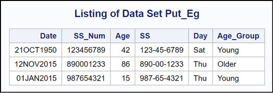
title “Listing of Data Set Put_Eg”;
proc print data=Put_Eg noobs;
run;
Explanation: This example demonstrates several uses of the PUT function. You first want to create a character variable (SS) from the numeric variable SS_Num. The built-in SAS format SSN11. formats a numeric value in Social Security form (i.e., adds leading zeros and hyphens). Next, by using the Downame3. format (Downame formats SAS dates to the names for the days of the week), you create a character variable containing the first three letters for each of the days. Finally, you create a format that groups Age into categories, and then you use the PUT function to create the variable Age_Group. This variable has values of ‘Young’ and ‘Older’ (plus ‘Error’ and ‘Missing’ if there are missing values and errors for Age). You would normally drop the variable SS_Num, keeping only SS, but it was not dropped so that you can see the original values of SS_Num in the listing.
Figure 15.7: Output from Program 15.7
Function Name: SUBSTRN (Newer Version of the SUBSTR Function)
What it does: Extracts a substring from a string.
Arguments: The first argument is a character value (one for which you want to extract a substring). The second argument is the starting position in the character value where you want to begin the substring. The third argument is the length of the substring that you want to extract. This last argument is optional. If you leave it out, the function returns characters from the starting position to the last non-blank character in the string.
Examples:
ID=’123NJ456’; Amount=’$12,456’;
substrn(ID,4,2) = NJ
substrn(ID,4) = NJ456
substrn(Amount,2) = 12,456
substr(ID,4,2) = NJ
Explanation: In the first example, you want to extract the state codes from the variable ID. The starting position is 4 and you want to extract two characters. In the second example, you leave off the third argument (the length) and the SUBSTRN function returns all the remaining characters in the string.
The variable Amount starts with a dollar sign, and you want to extract the digits (and commas) without the dollar sign.
Finally, the older SUBSTR function, used in this example, returns the same substring as the SUBSTRN function. There are some more advanced features that are available to you with the SUBSTRN function compared to the SUBSTR function, but these features are not used in most programs.
Very important point: If you do not define the length of the result of the SUBSTRN function, SAS gives it a default length equal to the length of the first argument (you cannot extract a substring longer than the original string). Every time you create a new variable using the SUBSTRN function, go back to the top of the DATA step and add a LENGTH statement, specifying the length of the substring variable.
Function Names: FIND and FINDC
What it does: FIND searches a string for a specific string of characters and returns the position in the string where this substring starts. If the substring that you are searching for is not found, FIND returns a 0.
FINDC searches a string for any one of the characters that you specify. It returns the position of the first character that it finds. As with the FIND function, if the search fails, the function returns a 0.
Arguments: The first argument in both of these functions is the character value that you are searching. For the FIND function, the second argument is the substring that you are looking for. For the FINDC function, the second argument is a list of individual characters that you are searching for. Both functions allow a third, optional argument (called a modifier) that allows these two functions to ignore case when doing their search.
There is also an optional third or fourth argument where you can specify a starting position for the search. If you use a modifier and a starting position, it doesn’t matter what order you place these two arguments. If you only use a modifier or a starting position, place it as the third argument. SAS figures out which is a modifier and which is a starting position because modifiers are always character values and starting positions are always numeric values.
Examples:
String1=’Good bad good’; String2=’NNyYnYNN’;
find(String1,’good’) = 10 (position of ‘good’ - lowercase)
find(String1,’good’,’i’) = 1 (the ‘i’ modifier says to ignore case)
find(String1,’ugly’,’i’) = 0 (did not find string ‘ugly’)
findc(String2,’Y’) = 4 (position of first uppercase ‘Y’)
findc(String2,’Y’,’i’) = 3 (the ‘i’ modifier says to ignore case)
findc(String2,’X’) = 0 (no ‘X’ in string)
findc(String1,’abcd’) = 4 (position of ‘d’)
Explanation:
FIND returns a 10 because the search is case-sensitive and the string ‘good’ starts in column 10.
FIND uses the ‘i’ (ignore case) modifier, so it finds the string ‘Good’ in the first position.
There is no string ‘ugly’, so the function returns a 0.
FINDC is searching for an uppercase ‘Y’ and finds it in position 4.
The ‘i’ modifier is used and the lowercase ‘y’ in position 3 is chosen.
There is no ‘x’ in the string, so the function returns a 0.
You are looking for an ‘a’, ‘b’, ‘c’, or ‘d’. The first character it finds in the string is the ‘d’ in position 4.
Note that these two functions replace the older INDEX and INDEXC functions (with added capability). There is also a third function, FINDW, that searches for words (strings bounded by word boundaries or other delimiters). Because this is not used as much as the other two functions, it was not included. You can find information about FINDW in the documentation.
Function Names: CAT, CATS, and CATX
What it does: You have already seen the concatenation operator (either || or !!) earlier in this chapter. Why do you need functions to concatenate strings? There are several advantages that these functions provide, as you will see in the examples that follow. CAT works in a similar manner to the concatenation operator. It takes a list of arguments and puts them together. CATS (pronounced Cat – S by most) is similar to CAT except that it strips leading and trailing blanks from each of the strings before putting them together (hence, the ‘S’ in the name). Finally, CATX does everything CATS does with one additional feature—it uses the first argument to the function as a separator between the strings. Note that the first argument to CATX can be more than one character.
Very important point: If you assign the result of a concatenation function to a variable and you do not define a length for this variable, SAS will assign a length of 200. This is different from the rule for the concatenation operator. When you use the operator, the length of the result is the sum of the lengths of each of the strings that you are concatenating.
Arguments: CAT and CATS: One or more character or numeric values. If you have variables in the form Variable1-VariableN, precede the list with the keyword OF. CATX: The first argument specifies one or more characters to use as separators between the strings. The second through last arguments are identical to the other CAT functions.
Examples:
Trail=’ABC   ‘;      Lead= ‘   ABC’;      Both=’   ABC   ‘;
C1=’A’;   C2=’B’;   C3=’C’;   C4=’D’;   C5=’E’;
cat(‘:’,Trail,Lead,’:’) = :ABC      ABC:
cats(‘:’,Trail,Lead,’:’) = :ABCABC:
catx(‘-’,’:’,Trail,Lead,’:’) = ABC-ABC:
catx(‘.’,908,782,1323) = 908.782.1323
cats(of C1-C5) = ABCDE
Explanation: In the first example, you are concatenating a colon, the two variables Trail and Lead, and another colon. Notice that Trail has three trailing blanks and Lead has three leading blanks. The result has six blanks between the letters.
The second example uses the CATS function. Therefore, there are no spaces between the letters.
In the third example, the first argument is a hyphen, so the resulting string is similar to the CATS example except you now have a hyphen between the letters.
The next CATX example demonstrates that the arguments to all the CAT functions can be numeric. Remember that the resulting string is a character value.
The last example takes the five variables (C1–C5) and creates a single string.
In practice, the two functions CATS and CATX are used the most. Notice that in the fourth example, the arguments are numeric values. CAT, CATS, and CATX can all take either character or numeric arguments. When you use numeric arguments, an automatic conversion from numeric to character is performed and there are no conversion messages in the log.
You will see later how the CATS function and the COUNTC function make for a very powerful duo.
Function Names: COUNT and COUNTC
What it does: COUNT counts the number of substrings in a character value. COUNTC counts the number of individual characters in a character value.
Arguments: The first argument in both functions is a character value. For the COUNT function, the second argument is the substring that you are searching for. For the COUNTC function, the second argument is a list of individual characters that you want to count. As with the CAT functions, if you have a list of character variables in the form Variable1-VariableN, precede the list with the keyword OF. Both functions can take a third, optional argument, the most popular being ‘i’ that means ignore case. (See the examples.)
Examples:
String=’Good bad good Good’; String2=’AABBxxxcccc’;
count(String,’good’) = 1 (the search is case-sensitive)
count(String,’good’,’i’) = 3 (‘i’ is the ignore case modifier)
countc(String2),’ABC’) = 4 (2 A’s and 2 B’s – the c’s are lowercase)
countc(String2,’ABC’,’i’) = 8 (the ‘i’ modifier is specified)
Explanation: The first example is searching for the string ‘good’ and it only finds it once.
Because the ‘i’ modifier is used in the second example, the function finds three occurrences of ‘good’.
In the first COUNTC example, there are a total of four uppercase As and Bs.
In the last COUNTC example, the ‘i’ modifier allows the four lowercase c’s to be counted as well.
In the example shown next, you have five variables (Q1–Q5), and you want to count the number of uppercase or lowercase Ys in these five variables. The classical approach to solving this problem is to create an array of the five ‘Q’ variables, set a counter to 0, and use a DO loop to test each of the five ‘Q’ variables for an uppercase or lowercase ‘Y’. Each time you find one, you increment the counter.
You can greatly simplify this problem by using the CATS function to place each of the five ‘Q’ values in a single character string. In the first observation, the result of the CATS function is the string ‘YyYnn’. You use this as the argument of the COUNTC function to count the number of uppercase or lowercase Y’s.
Program 15.8: Demonstrating the Combination of CATS and COUNTC
data Survey;
   input (Q1-Q5)($1.);
   Number_Y = countc(cats(of Q1-Q5),’Y’,’i’);
datalines;
YyYnn
NNnnn
NYNyy
;
title “Listing of Data Set Survey”;
proc print data=Survey noobs;
run;
Next time you find yourself creating an array and DO loops, consider if the problem can be solved using the method described in this example.
The output from Program 15.8 is shown below.
Figure 15.8: Output from Program 15.8
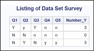
Imagine, a one-line solution to this problem!
What it does: Traditionally, it removes characters from a string. With the ‘k’ modifier, you can use this function to extract characters (for example, all digits) from a string. This is one of the most powerful character functions in the SAS arsenal—don’t skip this section!
Arguments: If you provide only one argument (a character value), this function removes blanks from the string. An optional second argument is a string of characters that you want to remove from the first argument. If you provide an optional third argument, you can specify character classes to remove from the first argument (such as all letters or all digits).
One of the most useful applications of this function is to use a ‘k’ (keep) modifier as the third argument. When you do this, the characters you list as the second argument and/or the characters that you specify with modifiers in the third argument are kept and all others are removed. The examples that follow should make this much clearer.
A list of some of the more useful modifiers is shown here:
|
Modifier |
Description |
|
‘a’ |
All upper- and lowercase letters |
|
‘d’ |
All digits |
|
‘p’ |
All punctuation (such as periods, commas, etc.) |
|
‘s’ |
All whitespace characters (spaces, tabs, linefeeds, carriage returns) |
|
‘i’ |
Ignore case |
|
‘k’ |
Keep the specified characters; remove all others (very useful) |
Examples:
String1=’abc def 123’; String2=’(908)782-1234’; String3=’120 Lbs.’;
compress(String1) = abcdef123 (one argument, default action remove blanks)
compress(String1,’0123456789’) = abc def (remove digits 0-9)
compress(String1,,’d’) = abc def (‘d’ modifier means remove all digits)
compress(String2,,’kd’) = 9087821234 (keep the digits)
compress(String3,,’kd’) = 120 (this is a character string, not a number)
input(compress(String3,,’kd’)) = 120 (a numeric value)
compress(String1,’ ‘,’kadp’) = abc def 123
Explanation:
Because there is only one argument, the COMPRESS function removes all blanks.
The second argument (all the digits 0 to 9) are removed. Back in SAS®8, the COMPRESS function did not have a third (modifier) argument, and this was the way you would need to remove all digits. You might see examples like this if you are looking at programs written before SAS®9.
It is important to notice that there are two commas in a row following the first argument. With only one comma, the function would think that ‘d’ is the second argument and you are trying to remove all ‘d’s from the string. Using two commas tells the function that ‘d’ is the third argument (modifier) and you want to remove all digits.
One of my favorites—keep the digits and throw everything else away.
Again, keep the digits. Here it is used to remove units from a value.
This example shows how to combine the INPUT function and the COMPRESS function to extract the numeric value when there are units (or other non-digit values) included. The result of the COMPRESS function is a character value, and the INPUT function performs the character-to-numeric conversion.
If you have character data that includes non-printing ASCII or EBCDIC characters, you can use an expression similar to this. Here you are keeping spaces, uppercase and lowercase letters, digits and punctuation, and throwing everything else away.
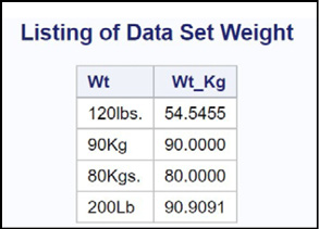
To further illustrate the power of the COMPRESS function, the next program shows how to deal with a quantity that contains different units (pounds and kilograms) and wind up with numeric values, all in the same units:
Program 15.9: Using the COMPRESS Function to Read Data That Includes Units
data Weight;
   input Wt $ @@;
   Wt_Kg = input(compress(Wt,,’kd’),12.);
   if findc(Wt,’L’,’i’) then Wt_Kg = Wt_Kg / 2.2;
datalines;
120lbs. 90Kg 80Kgs. 200Lb
;
title “Listing of Data Set Weight”;
proc print data=Weight noobs;
run;
You have weights that include units. Notice that the case of the units is not consistent, and the units might or might not include periods. The double trailing @ in the INPUT statement enables you to read multiple observations on one line of data (it prevents the program from going to a new line each time that the DATA step iterates). You use the COMPRESS function with the ‘kd’ modifier to extract the digits from each weight and the INPUT function to perform the character-to-numeric conversion. Although you call this Wt_Kg, it might actually be in pounds. Next, you check to see whether there is an upper- or lowercase ‘L’ in the units of the Wt variable with the FINDC function. If you find an ‘L’, you know the value is in pounds, so you divide Wt_Kg by 2.2 to convert the value to kilograms.
Here is the listing.
Figure 15.9: Output from Program 15.9
What it does: Takes a string apart (parses a string). The most common use is to extract the first and last name from a variable that contains the entire name (and possibly middle initial). The length of the result will be the same as the length of the first argument if you do not use a LENGTH statement to specify the length of the result.
Arguments: The first argument is the string that you want to take apart. The second argument specifies which “word” you want. The reason “word” is in quotation marks is because if you do not list one or more delimiters in the third argument, the default action of the SCAN function is to use blanks plus other characters such as commas, periods, hyphens, etc., as delimiters. In addition, the list of default delimiters is slightly different between ASCII and EBCDIC character sets. It is a good idea to specify exactly what delimiters you want as the optional, third argument. If the second argument is negative, the scan proceeds from right to left.
Examples:
String1=’Alfred E. Newman’; String2=’Cody, Ronald’; String3=’12-34-56’;
scan(String1,1,’ ‘) = Alfred (Specifying a blank delimiter)
scan(String1,2,’ ‘) = E. (The second word)
scan(String1,3) = Newman (Using the default delimiters that include blanks)
scan(String1,-1,’ ‘) = Newman (a negative second argument means scan right to left)
scan(String1,4) = ‘ ‘ (missing value – there is no fourth word)
scan(String2,1,’, ‘) = Cody (Specifying blanks and commas as delimiters)
scan(String3,2,’-’) = 34 (Specifying a hyphen as the delimiter)
Explanation:
By specifying a blank delimiter, the first word is ‘Alfred’.
The second word is ‘E’.
Because one of the default delimiters is a blank, the third word is ‘Newman’. It’s probably better to specify a blank as the delimiter if that is the only delimiter you want to use.
Using a -1 as the second argument is extremely useful in situations where you sometimes have first name and last name and at other times your name variable contains a middle name or initial. Using the -1 causes a right-to-left scan so that you can easily extract the last name in either of these situations.
Here you are looking for the fourth word in a string that only contains three words, so the function returns a missing value. This provides you with a useful tool for extracting words from strings when you don’t know how many words there are. You can extract each word in a DO loop and you know you are finished when the SCAN function returns a missing value.
Because blanks and commas are both used as delimiters in String2, you can specify both in the third argument. Any combination of commas and blanks will be treated as a single delimiter.
The SCAN function has many other uses besides extracting words from a string. By specifying the correct delimiter, you can parse other types of data.
When you use the SCAN function, you will probably want to use a LENGTH statement to declare a length for the result so that the result does not have the default length equal to the length of the first argument.
What it does: Sets all the arguments (character and/or numeric) to a missing value after the CALL statement executes. This routine is especially useful when you are writing a program where you need to initialize a large number of character or numeric variables to a missing value.
Arguments: As many character and/or numeric variables as you want. If you have a variable list in the form Variable1-VariableN, precede the list by the keyword OF.
Examples:
X1=1; x2=2; x3=3; C1=’ABC’; C2=’D’; C3=’Fred’; C4=’***’;
call missing(of X1-X3, of C1-C4);
After the call, the variables X1–X3 are all numeric missing values and the variables C1–C4 are all character missing values.
Function Names: NOTDIGIT, NOTALPHA, and NOTALNUM
There are many more NOT functions (NOTSPACE, NOTPUNCT, etc.), but these three are the most useful.
What it does: Determines the first position in a string that is not a digit (NOTDIGIT), an upper- or lowercase letter (NOTALPHA), a letter or digit (NOTALNUM). The functions all return the position of the first character in a string that is not in one of the specified categories. If all the characters in the string fit the category, the functions return a 0. One of the most useful applications of these functions is for data cleaning. If you have rules concerning allowable characters in a character variable (all digits, for example), you can use the appropriate NOT function to test if there are any characters that violate your condition.
Arguments: The first argument is a character value that you want to test. There is an optional second argument that is the starting position to begin the search. If the starting position is a negative number, go to the absolute value of the starting position and search from right to left.
Examples:
String1=’1234NJ’; String2=’abc123’; String3=’123456’;
notdigit(String1) = 5 (the position of the ‘N’)
notalpha(String2) = 4 (the position of the ‘1’)
notalnum(String2) = 0 (all characters are alphanumeric)
notdigit(String3) = 0 (all characters are digits)
notalpha(String2,-3) = 0 (start searching at position 3 and search right to left)
Explanation: In the first example, the ‘N’ is the first non-digit in the string. In the second example, the ‘1’ is the first non-letter in the string. In the third example, you get a 0 because NOTALNUM returns the position of the first character that is not a letter or digit. Because String2 contains only digits and letters, the function returns a 0. String3 contains all digits. Therefore, NOTDIGIT returns a 0. In the last example, a starting position of -3 is an instruction to go to position 3 in String2 and search from right to left. There are only digits from the third position to the beginning of the string, so NOTALPHA returns a 0.
Function Names: ANYDIGIT, ANYALPHA, and ANYALNUM
What it does: Searches a string for the first occurrence of a digit (ANYDIGIT), an upper- or lowercase letter (ANYALPHA), any digit or letter (ANYALNUM).
Arguments: The first argument is a character value that you want to test. There is an optional second argument that is the starting position to begin the search. If the starting position is a negative number, go to the absolute value of the starting position and search from right to left.
Examples:
String1=’1234NJ’; String2=’abc123’; String3=’123456’;
anydigit(String2) = 4 (position of the ‘1’)
anyalpha(String1) = 5 (position of the ‘N’)
anyalpha(String3) = 0 (no letters in the string)
anyalnum(String2) = 1 (position of the ‘a’)
Explanation: In the first example, the first digit in String2 is the ‘1’ in position 4. In the second example, the ‘N’ is the first letter and it is in position 5. In the third example, String3 does not contain any letters and the function returns a 0. In the last example, the first character ‘a’ is a letter or digit, so the function returns a 1.
What it does: Performs a find-and-replace operation. One popular use of this function is to help with address standardization, converting words like “Street” to “St.” and “Road” to “Rd.”
Arguments: The three arguments to the TRANWRD function are: 1) the string that you want to modify, 2) the ‘find’ string, and 3) the ‘replace’ string. Because the ‘replace’ string might be longer than the ‘find’ string, the default length for the result is 200. This fits with the general SAS rule that if the length returned by a function is longer than the length of the string argument, the default length will be 200.
Examples:
String1=’123 First Street’; String2=’Mr. Frank Jones Jr.’;
tranwrd(String1,’Street’,’St.’) = 123 First St.
tranwrd(String1,’Road’,’Rd.’) = 123 First Street
tranwrd(String2,’Jr.’,’ ‘) = Mr. Frank Jones
tranwrd(String2,’Mr.’,’ ‘) = Frank Jones (2 leading blanks)
Explanation: In the first example, “Street” is replaced by the abbreviation “St.” In the second example, because there is no “Road” in String1, nothing is changed. In the third example, you are substituting a blank for “Jr. “, removing “Jr.” from the string. In the last example, the resulting string has two leading blanks, one from converting “Mr.” to a blank and the other is the original blank that was between “Mr.” and “Frank.”
Having a knowledge of the SAS functions described in this chapter can save you immense time and effort. Some of the more obscure or complex SAS functions, including Perl regular expressions, were not covered here. Please refer to SAS for help online or one of the SAS Press books for information about these functions.
1. You have a SAS data set called Questionnaire2. It contains variables Subj (subject) and Q1–Q20 (numeric variables). Some of the values of Q1–Q20 might be missing values. Compute the following scores:
Score1 is the mean of Q1–Q10. Only compute Score1 if there are seven or more nonmissing values of Q1–Q10.
Score2 is the median of Q11–Q20. Compute Score2 only if there are five or fewer missing values in Q11–A20.
Score3 is the largest value in variables Q1–Q10.
Score4 is the sum of the two largest values in variables Q1–Q10.
To test your program, run the program below to create the Questionnaire2 data set:
Program for Problem Sets 9
data Questionnaire2;
input Subj $ Q1-Q20;
datalines;
001 1 2 3 4 5 1 2 3 4 5 1 2 3 4 5 1 2 3 4 5
002 . . . . 3 2 3 1 2 3 4 3 2 3 4 3 5 4 4 4
003 1 2 1 2 1 2 12 3 2 3 . . . . . . 4 5 5 4
004 1 4 3 4 5 . 4 5 4 3 . . 1 1 1 1 1 1 1 1
;
2. Modify the program from problem 1 to compute two new variables as follows: Mean_3_Large is the mean of the three largest values from Q1 to Q10. Mean_3_Low is the mean of the three lowest nonmissing values in variables Q1–Q10. To ensure a good bulletproof solution to this problem, do not compute a mean if there are fewer than three nonmissing values for variables Q1–Q10. That is not the case with the current data set, but it could happen. (Remember that the MEAN function ignores missing values.)
3. Run Program for Problem Sets 10 to create the data set Char_Data. Create a new SAS data set called Num_Data that has the three variables Date, Weight, and Height, which are numeric. Format Date with the DATE9. format. You will need to rename the variables derived from Char_Date so that those names can be used in the new data set. Hint: The RENAME= option is:
data-set-name(rename=(old1=new1 old2=new2, . . .));
Program for Problem Sets 10
data Char_Data;
length Date $10 Weight Height $ 3;
input Date Weight Height;
datalines;
10/21/1966 220 72
5/6/2000 110 63
;
4. Working with the data set Questionnaire2 (Problem 1), use CALL SORTN to compute the mean of the 12 highest scores in variables Q1–Q20. It is OK if some of the scores have missing values. You can perform a sort either in ascending order by listing the variables as Q1–Q20 or in descending order by listing the variables as Q20–Q1. Don’t forget the keyword OF in the CALL routine.
5. Run Program for Problem Sets 11 to create data set Oscar (which will be used for several of the remaining problems in this section).
Program for Problem Sets 11
data Oscar;
length String $ 10 Name $ 20 Comment $ 25 Address $ 30
Q1-Q5 $ 1;
infile datalines dsd dlm=” “;
*Note: the DSD option is needed to strip the quotes from
the variables that contain blanks;
input String Name Comment Address Q1-Q5;
datalines;
AbC “jane E. MarPle” “Good Bad Bad Good” “25 River Road” y n N Y Y
12345 “Ron Cody” “Good Bad Ugly” “123 First Street” N n n n N
98x “Linda Y. d’amore” “No Comment” “1600 Penn Avenue” Y Y y y y
. “First Middle Last” . “21B Baker St.” . . . Y N
;
Using the two length functions, compute the length of String, not counting trailing blanks and the storage length of String. Call these two variables L1 and L2.
6. Modify Program for Problem Sets 11 so that String is in uppercase and Name is in proper case. Use appropriate delimiters so that the name d’amore is spelled D’Amore.
7. Modify Program for Problem Sets 11 to create a new variable called Two_Three that contains the second and third characters in String. Be sure the length of Two_Three is 2.
8. Modify Program for Problem Sets 11 to include a new variable Yes_No. This variable should have a value of “Y” if the variable Comment contains the string “Good” (ignore case) and “N” if Comment does not contain the string “Good”. Yes_No should be a missing value if Comment is a missing value. In addition, create another variable called Count_Y that represents the total number of Ys in variables Q1–Q5. Hint: Use the CATS function to concatenate Q1–Q5.
9. First, run Program for Problem Sets 12. Modify this program to create a new numeric variable called Height that is the height in inches, computed from the variable Ht. Note: 1 inch = 2.54 cm.
Program for Problem Sets 12
Data How_Tall;
input Ht $ @@;
*Note: the @@ at the end of the INPUT statement allow you
to place several observations on one line of data;
datalines;
65inches 200cm 70In. 220Cm. 72INCHES
;
10. Using Program for Problem Sets 11, create a new variable called Last_Name (length 10) that is the last name computed from the variable Name. Hint: Remember that a minus value representing which “word” you want causes the function to scan from right to left. Also, convert Name to proper case before computing Last_Name.
11. Using Program for Problem Sets 11, convert the variable Address so that the words “Street” and “Road” are replaced by their abbreviations “St.” and “Rd.”