Chapter 16: Working with Multiple Observations per Subject
Because SAS processes one observation at a time, you need special programming tools when you want to analyze data where there are multiple observations per subject or any other grouping variable. For example, suppose you have a data set in which each observation represents a patient visit to a clinic. You record the patient ID, the date of the visit, and some health-related values. Some common programming tasks would include computing differences in values from visit to visit or differences between the first visit and the last visit for each patient. This chapter describes methods for solving problems of this type.
Useful Tools for Working with Longitudinal Data
Three useful programming tools for working with longitudinal data are first. and last. variables, the LAG and DIF functions, and retained variables. You will use all of these tools in the programs that follow.
Data set Clinic, shown below, is a collection of data on patients visiting a medical clinic. Some patients have only one visit—others have multiple visits. Data for each visit is stored in a separate observation. The following program creates the Clinic data set as well as a listing.
Program 16.1: Creating the Clinic Data Set
data Clinic;
   informat Date mmddyy10. PtNum $3.;
   input PtNum Date Height Weight Heart_Rate SBP DBP;
   format Date date9.;
datalines;
001 10/21/2015 68 190 68 120 80
001 11/25/2015 68 195 72 122 84
002 9/1/2015 72 220 76 140 94
003 5/6/2015 63 101 78 118 66
003 7/8/2015 63 106 76 122 70
003 9/1/2015 63 105 77 116 68
;
title “Listing of Data Set Clinic”;
proc print data=Clinic;
   id PtNum;
run;
Here is the listing.
Figure 16.1: Output from Program 16.1
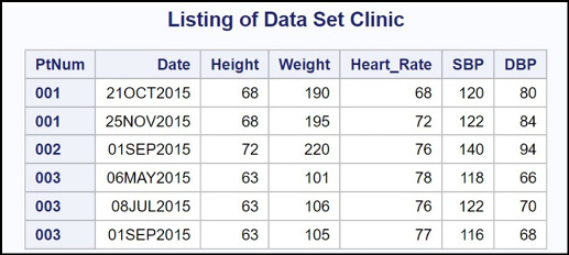
Patient 001 had two visits, patient 002 had one visit, and patient 003 had three visits.
Describing First. and Last. Variables
With this type of data, one of the first things you want to do is determine when you are processing the first observation and when you are processing the last observation for each patient. For this example, you want to first sort the data set by PtNum and Date. (Note: Sorting by date is not necessary here because visits are in date order for each patient. It is just a precaution in case a visit is out of order.) Next, you create a new data set (let’s call it Clinic_New), as follows.
Program 16.2: Creating First. and Last. Variables
proc sort data=Clinic;
   by PtNum Date;
run;

data Clinic_New;
   set Clinic;
   by PtNum;
   file print;
   put  PtNum= Date= First.PtNum=  Last.PtNum=;
run;
The key is to follow the SET statement with a BY statement. Doing this creates two temporary variables, First.PtNum and Last.PtNum. These variables are automatically dropped from the output data set. They only exist as the DATA step is processing. That is the reason that you use a PUT statement to examine these variables. Using PROC PRINT will not work because these two variables are temporary and are not in data set Clinic_New.
The statement FILE PRINT is an instruction to send the results of the PUT statement to the RESULTS window, not to the SAS log, which is the default location.
Here is the output from Program 16.2.
Figure 16.2: Output from Program 16.2
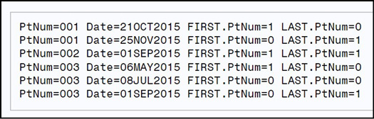
The variable First.PtNum is equal to 1 for the first visit for each patient and 0 otherwise—the variable Last.PtNum is equal to 1 for the last visit for each patient and 0 otherwise. Let’s see how you can use the First. and Last. variables in a program.
Computing Visit-to-Visit Differences
The first task is to compute visit-by-visit changes in the heart rate and the systolic and diastolic blood pressure for each patient. Here is the program.
Program 16.3: Computing Visit-to-Visit Differences in Selected Variables
proc sort data=Clinic;
   by PtNum Date;
run;

data Diff;
   set Clinic;
   by PtNum;
   if First.PtNum and Last.PtNum then delete;
   Diff_HR = dif(Heart_Rate);
   Diff_SBP = dif(SBP);
   Diff_DBP = dif(DBP);
   if not First.PtNum then output;
run;

title “Listing of Data Set Diff”;
proc print data=Diff;
   id PtNum;
run;
It makes no sense to compute differences for patients with only one visit. Patients with one visit have both variables, First.PtNum and Last.PtNum, equal to 1 (it is both the first and last visit), so you delete these observations. You use the DIF function to compute differences in heart rate, systolic blood pressure, and diastolic blood pressure for each patient (you can review the DIF function in Chapter 15). For the first visit for each patient (not including the first patient), you are actually computing the difference in each variable based on the last value from the previous patient and the current value. This is OK. You are only outputting observations for the second through last visit for each patient. You might be tempted to compute the difference values conditionally (that is, only for the second through last visits). This does not work. Remember that the DIF function returns the value of its argument the last time the function executed. If you do not execute the DIF function for the first visit for each patient, when you finally execute it, the function will return the value from the last time the function executed, giving you the last value from the previous patient. If you like, on the first visit for each patient, after you execute the DIF function, you can set the difference variables to a missing value.
Here is the output from Program 16.3.
Figure 16.3: Output from Program 16.3
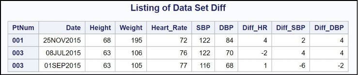
Each observation shows differences between the current visit and the previous visit.
Computing Differences between the First and Last Visits
The next task is to compute the difference in the three variables (Heart_Rate, SBP, and DBP) from the first visit to the last visit. The primary tool to solve this problem is to use retained variables. As you (hopefully) remember, variables defined in assignment statements are automatically set to a missing value at the top of the DATA step. By using a RETAIN statement, you can instruct the program not to set these variables to a missing value—you are retaining them. This is one way to have the program “remember” a value from some previous observation. If you set a retained variable equal to a value from the first visit, then that retained value will be available when you are processing the last visit, enabling you to compute a difference score. The next program uses this strategy.
Program 16.4: Computing Differences Between the First Visit and the Last Visit
proc sort data=Clinic;
by PtNum Date;
run;
data First_Last;
set Clinic;
retain First_Heart_Rate First_SBP First_DBP;
by PtNum;
if First.PtNum and Last.PtNum then delete;
if First.PtNum then do;
First_Heart_Rate = Heart_Rate;
First_SBP = SBP;
First_DBP = DBP;
End;
if Last.PtNum then do;
Diff_HR = Heart_Rate - First_Heart_Rate;
Diff_SBP = First_SBP - SBP;
Diff_DBP = First_DBP - DBP;
output;
end;
run;
title “Listing of Data Set First_Last”;
proc print data=First_Last;
id PtNum;
run;
You use a RETAIN statement for the three variables that will contain the value of heart rate, SBP, and DBP from the first visit.
Delete patients with only one visit.
When you are processing the first visit for each patient, set each of the retained variables equal to the value of heart rate, SBP, and DBP, respectively.
When you reach the last visit for each patient, compute the difference of the current value minus the value from the first visit. Also, output an observation to data set First_Last.
Here is the listing.
Figure 16.4: Output from Program 16.4
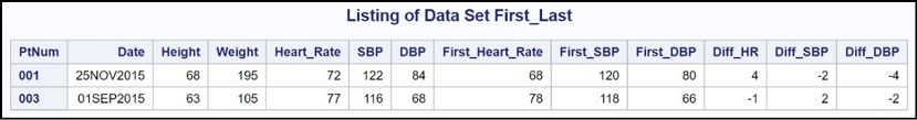
Each observation represents the last visit for each patient (who had more than one visit) and the differences between the first visit and the last visit.
Counting the Number of Visits for Each Patient
Another common task is to count the number of observations (visits, in this example) for each subject or other grouping variable. One of the most straightforward ways to accomplish this is to initialize a counter to 0 when you are processing the first visit for each patient, increment the counter for each visit, and output the patient number and visit count when you are processing
the last visit for each patient. The next program uses this technique to create a data set of patient numbers and visit counts:
Program 16.5: Counting the Number of Visits for Each Patient
proc sort data=Clinic;
   by PtNum;
run;

data Counts;
   set Clinic;
   by PtNum;
   if First.PtNum then N_Visits=0;
   N_Visits + 1;
   if Last.PtNum then output;
run;

title “Listing of Data Set Counts”;
proc print data=Counts;
   id PtNum;
run;
Because you follow the SET statement with a BY statement, you have the temporary variables First.PtNum and Last.PtNum at your disposal. When you are processing the first visit for each patient, you set the variable N_Visits equal to 0. Then, for every visit (observation), you use a SUM statement to add one to the counter.
Because it is so important, let’s take a minute to review the properties of the SUM statement. If you had used an assignment statement like this:
N_Visits = N_Visits + 1;
The variable N_Visits would be set to a missing value for each iteration of the DATA step. A SUM statement differs from an assignment statement because it is in the form:
Variable + Expression;
There is no equal sign in this expression. There are three very important properties of a SUM statement:
● First, the variable is automatically retained.
● Second, the variable is initialized to 0.
● Third, if the expression results in a missing value, it is ignored.
The bottom line is that the SUM statement as used here is simply a counter.
When you are processing the last visit for each patient (Last.PtNum is true), you output an observation. This observation contains the heart rate, the systolic and diastolic blood pressure, and the number of visits for each patient. Here is the listing.
Figure 16.5: Output from Program 16.5
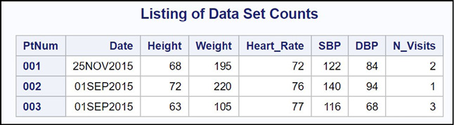
The variable N_Visits represents the number of visits for each patient.
You need special programming tools to analyze data for which you have multiple observations for each value of a BY variable. This chapter described some of these tools.
1. First run Program for Problem Sets 13 to create the Clinic data set. Next, write a DATA step that computes the visit-to-visit differences in Heart_Rate and Weight. Be sure to omit any patient with only one visit and only output an observation for the second through last visits for each patient. Careful, the data set is not sorted by Subj or Date.
data Clinic;
informat Date mmddyy10. Subj $3.;
input Subj Date Heart_Rate Weight;
format Date date9.;
datalines;
001 10/1/2015 68 150
003 6/25/2015 75 185
001 12/4/2015 66 148
001 11/5/2015 72 152
002 1/1/2014 75 120
003 4/25/2015 80 200
003 5/25/2015 78 190
003 8/20/2015 70 179
;
2. Using the Clinic data set from Problem 1, create a new data set (New_Clinic) that has one observation per subject. This one observation should include the number of visits for each subject (N_Visits) and the change in heart rate and weight from the first visit to the last visit. Omit any subject with only one visit.
3. Try to answer this question without running Program for Problem Sets 14 first. What is the value of Last_x in each of the five observations?
data Tricky;
input x;
if x gt 5 then Last_x = lag(x);
datalines;
6
7
2
10
11
;
4. What’s wrong with this program (assume that you have just run Program for Problem Sets 13)?
1 data New;
2 set Clinic;
3 if first.Subj then First_Wt = Weight;
4 if last.Subj then Diff-Wt = Weight – First_Wt;
5 run;