In the last chapter, you saw how to use the Import Data facility on the Utilities tab to import data. In this chapter, you will see how to use several of the most useful tasks as well as the Query tool on the Utilities tab.
It is worth repeating this note from the previous chapter: In this book, as well as in SAS Studio, you will see the terms SAS data set and table used interchangeably as well as these other equivalent terms: variables are also called columns and observations are called rows.
Using the List Data Task to Create a Simple Listing
SAS Studio has dozens of built-in tasks. If you expand the Tasks tab and click the Data tab, you will see the following.
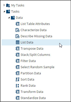
You can use the List Data task to create a listing of your data set. To demonstrate this, we are going to use the built-in SASHELP data set called Fish. This data set contains information about several species of fish, including weight, length, and width. To create a listing of this data set, expand the list of Data tasks and double-click List Data. This brings up the screen shown in Figure 4.2.
Figure 4.2: The List Data Task Settings Screen
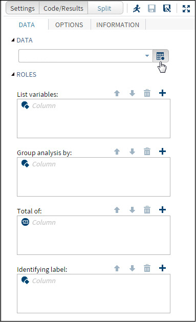
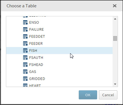
You can click the icon at the top right part of this screen (shown in the figure with a hand pointing to it) to select the library and data set you want to list. Because you want a listing of SASHELP.Fish, select this data set and click OK.
Figure 4.3: Selecting the Fish Data Set in the SASHELP Library
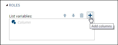
The next step is to click the plus sign to select which variables you want to include in your listing. (See Figure 4.4.)
Figure 4.4: Adding Columns (Variables)
When you see the list of variables, you can select them in the usual way. (See the instructions below.)
To select variables from a list, use one of these two methods: 1) Hold the Ctrl key down and select the variables that you want; or 2) Click one variable, hold the Shift key down, and click another variable—all the variables from the first to the last will be selected.
In this example, you are selecting Species, Weight, Height, and Width.
Figure 4.5: Selecting Variables to List
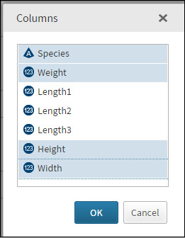
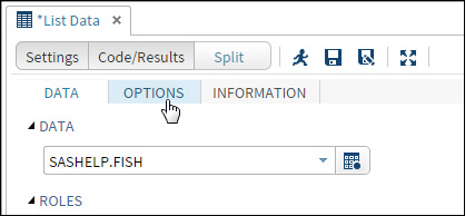
Click OK when you are finished. You can create the listing now or click the OPTIONS tab to customize the listing.
Figure 4.6: Using the OPTIONS Tab to Customize the Listing
Here is the list of options available for the List Data task.
Figure 4.7: Options for the List Data Task
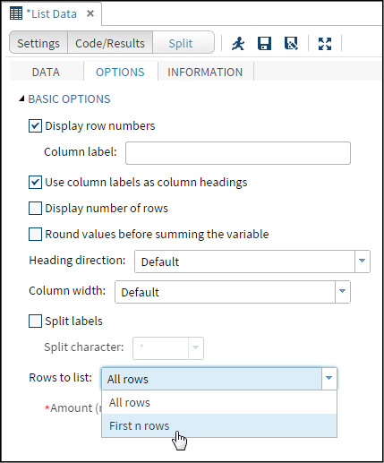
You can check or uncheck the Display row numbers box to include the Obs column in the listing or to omit it. You have a choice of using column labels or column names in the listing. If you are a programmer, then you will probably want to see column names as headings. If you are creating the listing for a report, then you will probably want to see column labels.
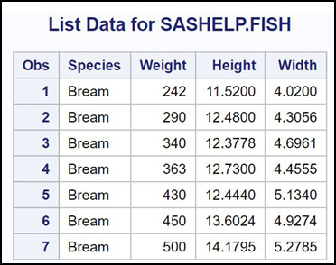
The option displayed at the bottom of Figure 4.7 gives you the choice of listing all the rows of the table or the first n rows. In this example, you want to see the first seven rows of the Fish data set. This is shown in the next figure.
Figure 4.8: Requesting the First Seven Rows to Be Displayed
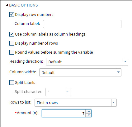
Clicking the Run icon generates the following listing.
Figure 4.9: Listing of the First Seven Rows of the Fish Data Set
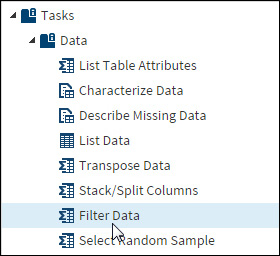
Another useful task is to filter the table—that is, you select rows that meet predefined criteria. To do this, double-click Filter Data in the task list.
Figure 4.10: Selecting Filter Data from the Data List
This brings up the following.
Figure 4.11: Selections for Filtering Data
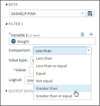
You select the data set as before. Next, you select a variable and a condition for your filter. In this example, you are selecting Weight as your variable and Greater than as your condition. You can now enter a value for the filter. In this example, you want to see rows in the table where the variable Weight is greater than 1,100.
Figure 4.12: Selecting Rows Where the Weight Is Greater Than 1,100
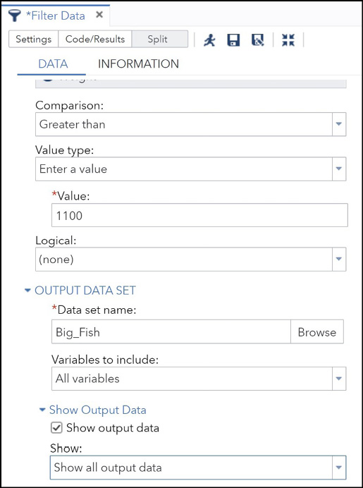
You can also expand the OUTPUT DATA SET option to override a default data set name. In most cases, you will want to supply your own data set name. Here you are naming the data set Big_Fish. You can also check or uncheck the Show Output Data box. Selecting it (as in this example) generates a listing of the filtered data set.
Notice that there is no comma in the number 1100 in the figure above. A comma would generate an error.
Figure 4.13: Listing of the Filtered Data Set (Big_Fish)

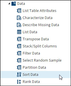
To sort a SAS data set by a variable, select Sort Data from the list.
Figure 4.14: The Sort Data Task
Just as in the previous tasks, you can now choose a data set and options.
Figure 4.15: Selecting a Data Set and Variables for the Sort
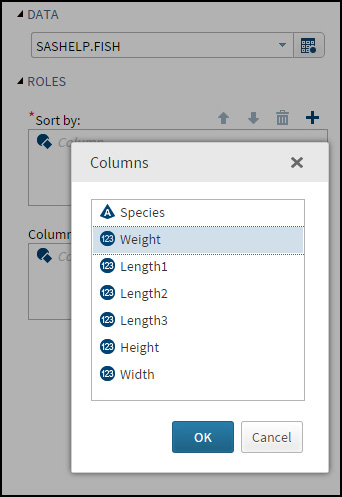
You are starting with the SASHELP.Fish data set and requesting a sort based on the variable Weight. You can also choose columns to drop in this operation.
Figure 4.16: Selecting Columns to Drop
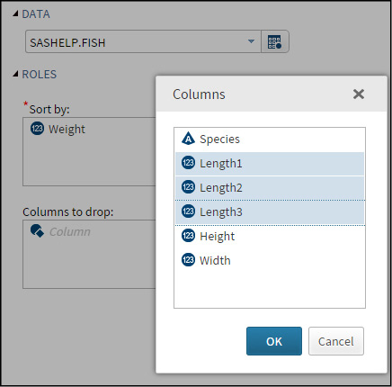
In this example, you are dropping the three Length variables.
Before you execute the sort, there are several options that you should consider. Click the OPTIONS tab to see these options. The default sort order is ascending (from smallest to largest). However, in this case, you want to see the heavier fish at the top of the list, so you choose Descending as the sort order.
Figure 4.17: Selecting a Descending Sort
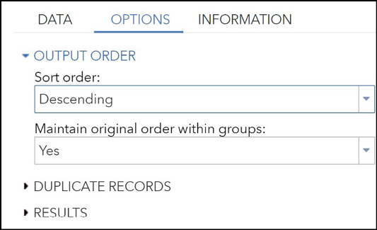
Expand the RESULTS option to either sort in place or create a new data set with the sorted data.
CAUTION: Sorting in place replaces the original data set with the sorted data. If you drop columns, they will no longer be in the sorted data set.
In this example, you do not want to sort the original table—you want to create a new data set called Sorted_Fish:
Figure 4.18: Naming the Output Data Set

Click the Run icon to see the following screen.
Figure 4.19: Result of Executing the Sort
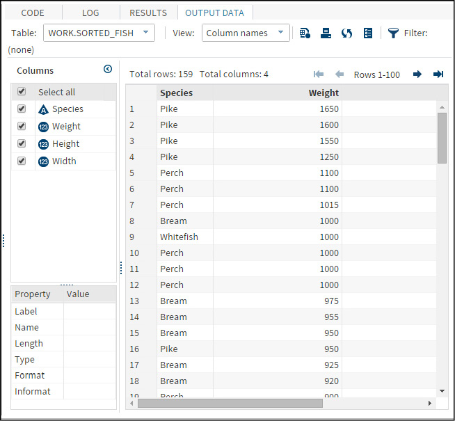
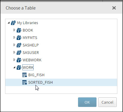
To see a nicer listing of this data set, go back to the List Data selection and proceed as you did in the first section of this chapter. Once you have opened the List Data task, choose a table to display and any options that you want. We will see that process below.
Figure 4.20: Choose a Table to List
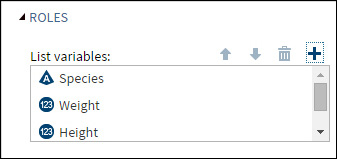
Next, choose which variables to include in the listing.
Figure 4.21: Choosing Variables to List
Finally, select any options that you want. In this example (see Figure 4.22), you want to see the first eight rows of the table.
Figure 4.22: Option to List the First Eight Rows of the Table

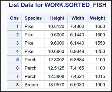
Here is the listing.
Figure 4.23: First Eight Rows of the Sorted_Fish Data Set
You can download this listing as an HTML or PDF by clicking the appropriate icon at the top of the results window (as shown below).
Figure 4.24: Icons to Download HTML or PDF Files
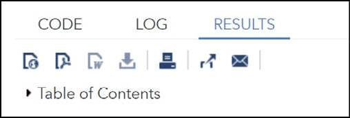
The left-most icon allows you to download the listing as an HTML file. The icon to the right of the HTML icon downloads the listing as a PDF file.
To create an RTF (rich text format) file, first click the SAS Studio Options icon.
Figure 4.25: Click More Application Options

Click Preferences, then Results, and then check RTF. HTML and PDF are already chosen by default. (Note: These preferences remain in effect unless you change them later.)
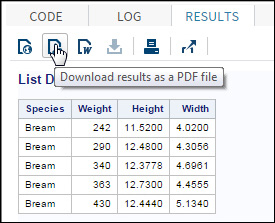
In Figure 4.26, you are downloading a PDF file.
Figure 4.26: Downloading a PDF File
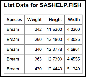
Here is a listing of the PDF file.
Figure 4.27: Listing of the PDF File
Joining Tables (Using the Query Window)
The last topic in this chapter describes how to use the Query utility to join two tables. Two data sets, ID_Name and Grades, were created to explain how the joining process works. Figure 4.28 shows a listing of these two data sets.
Figure 4.28: Listing of Data Sets ID_Name and Grades
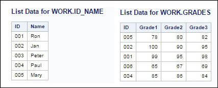
There are several features of these two data sets that are important for you to notice. Note the following: The data set ID_Name is sorted in ID order—in the data set Grades, it is not. This does not cause a problem—the Query tool automatically sorts the data sets. Also, ID 003 is in data set ID_Name and not in data set Grades; ID 006 is in Grades but not in ID_Name. The goal is to join these two tables based on the ID column.
If you want to play along with this demonstration, you can run the program shown next to create these two tables.
Program 4.1: Program to Create Data Sets ID_Name and Grades
data ID_Name;
   informat ID $3. Name $12.;
   input ID Name;
datalines;
001 Ron
002 Jan
003 Peter
004 Paul
005 Mary
;
data Grades;
   informat ID $3.;
   input ID Grade1-Grade3;
datalines;
005 78 80 82
002 100 90 95
001 99 95 98
006 65 67 69
004 85 86 84
;
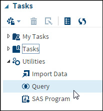
The first step in joining these two tables is to select Query from the Utilities tab.
Figure 4.29: The Query Task in the Utilities Tab
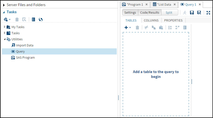
This brings up the following screen.
Figure 4.30: The Query Window
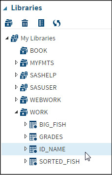
The next step is to open the Libraries tab and find the Work library.
Figure 4.31: Locate the Two Tables in the Work Library
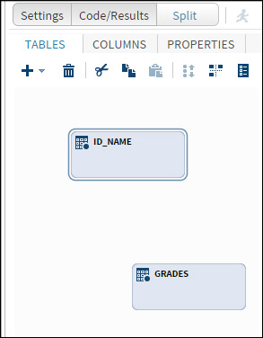
Click each file and drag it into the Query window. (If you drag the second file on top of the first file, SAS Studio automatically assumes that you want to perform a join operation.)
Figure 4.32: Drag the Two Files into the Query Window
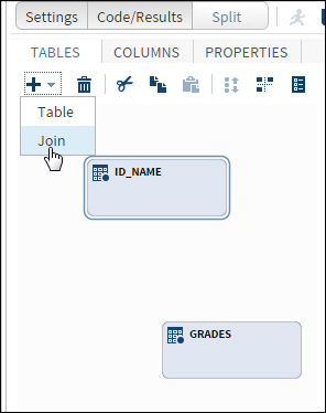
In the menu on the TABLES tab, select Join (unless you dragged the second file on top of the first, in which case the Query tool assumes that you want a join).
Figure 4.33: Selecting Join in the Menu
This brings up the following screen.
Figure 4.34: Getting Ready to Join the Two Tables

Select ID_Name for the Left table and Grades for the Right table. For Join type, select Inner join.
Figure 4.35: Selecting the Two Tables and Inner Join

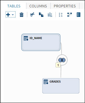
Click Save. You now see the two tables with a Venn diagram that represents an inner join. If you are familiar with SQL, you already know the four types of joins. For those readers who are not, here is the explanation.
Because some IDs are only in one table, you have some decisions to make about how you want to handle the join. The most common join, selected in this example, is an inner join. This type of join includes only those rows where there is a matching ID in both files. An outer join includes all rows from both tables (with missing values in the rows from the table that does not contain an ID). Finally, the other two joins are a left join and a right join. In a left join, all IDs from the left table are included even if there isn’t a matching ID in the right table. In a right join, all IDs from the right table are included even if there isn’t a matching ID in the left table.
Figure 4.36: Venn Diagram Showing an Inner Join of the Two Tables
The next step is to name the columns that you want to use to join the two tables. In this example, because ID is in both tables, the Query tool automatically selects ID for the join variable. You are free to select any variable from each file to construct the join, even if the variable names are not the same in the two files.
Figure 4.37: Selecting the Join Conditions

Next, select which columns you want in the joined table. To do this, click the COLUMNS tab. Select the columns in the usual way, and drag them to the Add columns area.
Figure 4.38: Selecting Columns for the Final Table

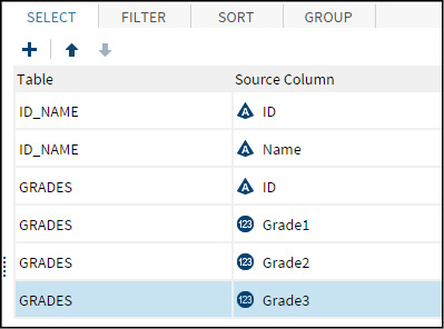
The figure below shows the final list of columns in the joined table.
Figure 4.39: Variables in the Joined Table
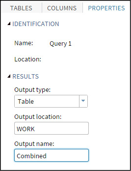
The last step is to click the PROPERTIES tab and indicate whether you want SAS to create a table or a report. If you choose a table, you can name the location (the Work library in this example) and the table name.
Figure 4.40: Options in the PROPERTIES Tab
Clicking the Run icon finishes the join. A snapshot view of the resulting table is produced.
Figure 4.41: View of the Resulting Table

You can use the List Data task to create a listing of the resulting table. It is shown in Figure 4.42.
Figure 4.42: Listing of Combined Data Set
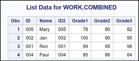
Because this was an inner join, only those IDs that were in both tables are listed in the final table.
Only a few of the more popular data tasks were described in this chapter. Once you get the knack of running a task, you should feel confident in trying out some of the other data tasks in the list. The decision to use a task or write a SAS program is a personal choice. For those with programming experience, writing a program might be the way to go—for those folks who are new to SAS and just want to get things done, using the tasks is a great way to go. Or you can do both! Use a task or a utility to get the basic program written for you, and then take that and edit it to do more.