Chapter 7: An Introduction to SAS Programming
This section of the book is dedicated to teaching you how to write your own programs in SAS. Perhaps you have some programming experience with other languages, such as C+, Python, or Java. This is both an advantage and a possible disadvantage. The advantage is that you understand how to think logically and use conditional logic, such as IF-THEN-ELSE statements and DO loops. On the other hand, SAS is somewhat unique in the way it reads and processes data, so you need to “re-wire” your brain and start to think like a SAS programmer.
SAS programs consist of DATA steps, where you read, write, and manipulate data and PROC (short for procedure) steps, where you use built-in procedures to accomplish tasks such as writing reports, summarizing data, or creating graphical output. DATA steps begin with the keyword DATA and usually end with a RUN statement. PROC steps begin with the word PROC (did you guess that?) and end with either a RUN or QUIT statement (or both).
SAS statements all end with semicolons. This is a good place to mention that one of the most common programming mistakes, especially with beginning SAS programmers, is to forget a semicolon at the end of a statement. This sometimes leads to confusing error messages.
The SAS Studio Programming Windows
When you open up SAS Studio, you see three tabs: CODE, LOG, and RESULTS. (See Figure 7.1 below.)
Figure 7.1: The Three SAS Studio Windows
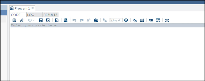
The CODE window is where you enter your SAS program. When you run a SAS program, the LOG window displays your program, any syntax errors detected by SAS, information about data that was read or written out, and information about real time and CPU time used. The RESULTS window is where any SAS output appears. You can navigate among the three windows by clicking the appropriate tab.
Let’s first write a simple program and then follow what happens when it runs. Suppose you want a program that converts temperatures from Celsius to Fahrenheit. It is a good idea to start your program by writing a comment statement. As part of the comment, you should, at a minimum, state the purpose of the program. In a more formal setting, you might also include information such as who wrote the program, the date on which it was written, and the location of input and/or output files. One way of writing comments in SAS programs is to start the comment with an asterisk and end it with a semicolon.
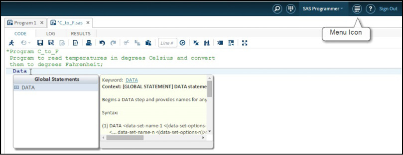
The next line is a DATA statement where you give a name to the data set you are going to create. Look what happens as you start to write the word DATA:
Figure 7.2: Illustrating the Autocomplete Feature of SAS Studio

As you type certain keywords in the CODE window, context-sensitive boxes pop up to show you syntax and options that are available for the statement that you are writing. If you are a more advanced user who does not need this syntax help, you can turn it off by clicking the menu icon (on the top right of the screen) as follows:
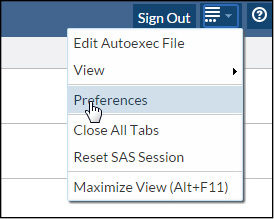
Figure 7.3: SAS Studio Options
Choose the Preferences tab on this menu.
Figure 7.4: Selecting SAS Studio Preferences
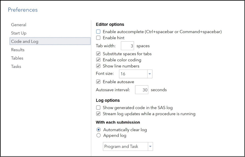
Under the Editor tab, select (or deselect) Enable autocomplete and click Save.
Figure 7.5: Select or Deselect Autocomplete
The complete program is listed below.
Program 7.1: Program to Read Temperatures in Degrees Celsius and Convert Them to Fahrenheit
*Program C_to_F
 Program to read temperatures in degrees Celsius and convert
 them to degrees Fahrenheit;

Data Convert;
   infile “~/MyBookFiles/celsius.txt”;
   input Temp_C;
   Temp_F = 1.8*Temp_C + 32;
run;

title “Temperature Conversion Chart”;

proc print data=Convert;
   var Temp_C Temp_F;
run;
This program starts with the keyword DATA. In this program you name the data set Convert. The rules for naming data sets and many other SAS names (such as variable names) are as follows:
In SAS, data set names and variable names must start with a letter or underscore. They can contain a maximum of 32 characters, and the remaining characters must be letters, digits, or underscores.
The following tables show examples of valid and invalid SAS names.
|
Valid SAS Names |
|
My_Data |
|
HeightWeight |
|
X123 |
|
_123 |
|
Price_per_pound |
|
Invalid SAS Names |
|
|
My Data |
Contains an invalid character (space) |
|
123xyz |
Starts with a digit |
|
Temperature-Data |
Contains an invalid character (-) |
|
Group% |
Contains an invalid character (%) |
In SAS, variable names are not case-sensitive. However, the case that you use the first time you reference a variable is used in SAS output, regardless of how you write the variable name in other locations in the program.
The INFILE statement tells the program where the raw data is located (use a different statement if you have cooked data). In this book, all the data from your hard drive was uploaded to the folder MyBookFiles (described in Chapter 3). In this author’s account, the actual location for this file is /home/ronaldcody/MyBookFiles/Celsius.txt. A shortcut to refer to this file is to place a tilde (~) to represent the home directory, as shown in the INFILE statement above.
File names in Windows are not case sensitive; however SAS Studio is running in a Linux operating system on the SAS® Cloud platform. File names are case sensitive in Linux (also in UNIX).
For example, if you wrote Celsius.txt instead of celsius.txt the program would not be able to find the file. This author was just reminded of that fact when he ran a program and was momentarily confused as to why the error message saying that the physical file could not be found was shown in the SAS LOG.
If you want to run the programs in this book, remember that you can download all of the programs and data sets from the following location:
support.sas.com/cody
Once you arrive at this location, locate this book and click the link “Example Code and Data.” This action downloads a ZIP file containing all the programs and data files in the book to your hard drive. You will want to extract these files to your hard drive and upload them to the MyBookFiles folder in SAS Studio (or whatever name you choose). You will also want to perform a similar action on the files and programs needed for the end-of-chapter problems. The solutions at the end of this book use a folder called Problems for these files and programs. You can use this name or any other name of your choosing.
The INPUT statement is an instruction to read data from the celsius.txt file. This text file contains one number per line and is listed below.
File 7.1: celsius.txt
0
100
20
This INPUT statement uses one of three methods of reading data, called list input. When you use list input, you can read data values separated by blanks (the SAS default delimiter) or other delimiters such as commas. Information about how to process data with delimiters other than blanks is presented in the next chapter.
Following the INPUT statement, you use an assignment statement to code the formula for the Celsius to Fahrenheit conversion. As with most programming languages, the calculation to the right of the equal sign is assigned to the variable name to the left of the equal sign. In this example, the calculated value is assigned to the variable Temp_F.
You use an asterisk to indicate multiplication, a forward slash for division, plus and minus signs for addition and subtraction, and two asterisks for exponentiation. Exponentiation is performed first, multiplication and division next, followed by addition or subtraction. You can always use parenthesis to determine the order of operations.
The DATA step ends with a RUN statement. In this program, the statements in the DATA step and PROC step are indented. This is not necessary, but it makes the program easier to read. It is also possible to place more than one SAS statement on a single line, as long as each statement ends with a semicolon. However, this practice is discouraged because it makes it difficult to read and understand the program. Finally, a SAS statement can use as many lines as necessary, such as the comment statement in this program. Just remember to end the statement with a semicolon.
SAS Studio has an auto formatting feature that you can use to automatically format your SAS programs. After you have written your program in the CODE window, click the AUTOFORMAT icon at the top of the EDITOR window (as shown in the figure below).
Figure 7.6: Activating the Auto Formatting Feature of SAS Studio

The result is a nicely formatted program. You can use CTRL+Z to undo the formatting in case you don’t like the result.
Unlike most programming languages, the SAS DATA step is actually an automatic loop: The first time the INPUT statement executes, the program reads a value from the first line of data. It then computes the corresponding Fahrenheit temperature according to your formula and adds the newly created variable to the data set SAS is creating. Your next statement is a RUN statement that marks the end of the DATA step. Two things happen at this point: First, the program automatically outputs an observation (containing the variables Temp_C and Temp_F) to the output data set that you named Convert. Next, the program performs its implied loop by returning to the top of the DATA step to execute the INPUT statement again. On the second iteration of the DATA step, SAS reads data from the second line of data. Each time the DATA step iterates, the INPUT statement goes to a new line of data (unless you give it special instructions not to). In this example, the DATA step stops when it tries to read the fourth line of data from the file and encounters an end-of-file marker. At this point, your SAS data set Convert contains three observations.
You use PROC PRINT to list the contents of your SAS data set. In this example, you specify the name of the SAS data set using the procedure option DATA= . You can specify one or more title lines with a TITLE statement. You can place a TITLE statement before or after the PROC statement. When you specify a title, that title remains in effect until you replace it with another TITLE statement. In this program, you placed the TITLE statement between the DATA and PROC steps, a location referred to as open code.
You use a VAR statement to specify which variables you want to include in your report. The order you use to list the variables on the VAR statement is the order that PROC PRINT will use to print the results. If you leave out a VAR statement, PROC PRINT will print every variable in your data set in the order they are stored in the data set. You end the PROC step with a RUN statement.
You are now ready to run the program. You do this by clicking the RUN icon as shown in Figure 7.7.
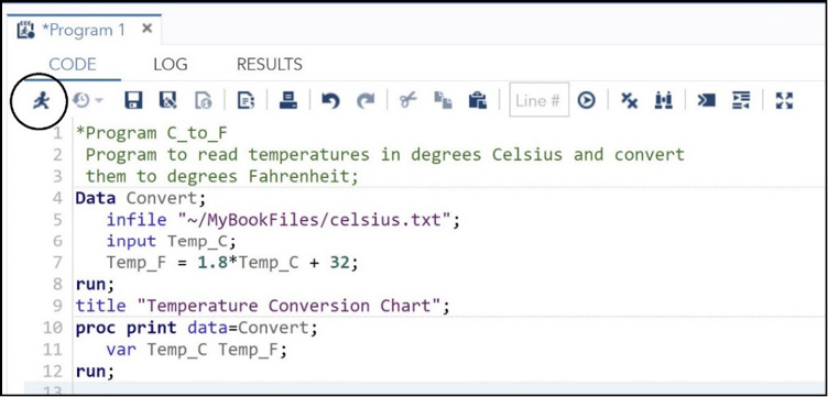
SAS Studio now shows you the results.
Figure 7.8: The RESULTS Window
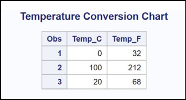
Be default, SAS lists all rows (called observations in SAS terminology) and all columns (called variables by SAS). It also includes an Obs (observation number) column. A quick examination of the output shows that the program worked correctly. However, you should always look at the SAS log, even when you have output that seems to be correct. To examine the log, click the LOG tab. Below is a listing of the log.
Figure 7.9: The LOG Window
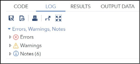
The first part of the log shows there were no errors or warnings. You can click any of these items to display any errors, warnings, or notes. Excerpts from the remaining log follow.
The first section shows your program, along with information about your input data file. Notice that SAS Studio added an OPTIONS statement to your program. This statement controls what information is displayed in the log and how the data appears in the RESULTS window.
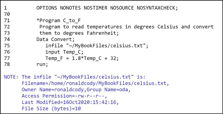
Next, you see that three records (lines) were read from the input file.

Finally, you see that PROC PRINT read three observations. You also see the real and CPU times.

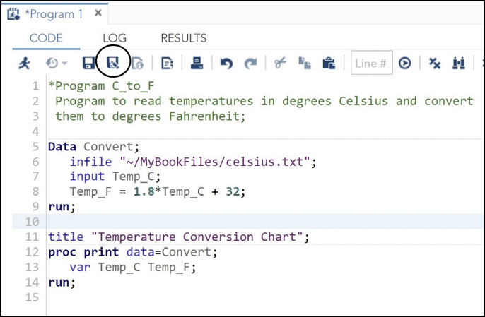
Before you close your SAS session, you should save your program so that you can work on the program later or, if it is finished, to save it. From the CODE tab, select the icon for SAVE AS:
Figure 7.10: The SAVE AS Icon
This brings up the following screen.
Figure 7.11: Saving Your Program in My Folders
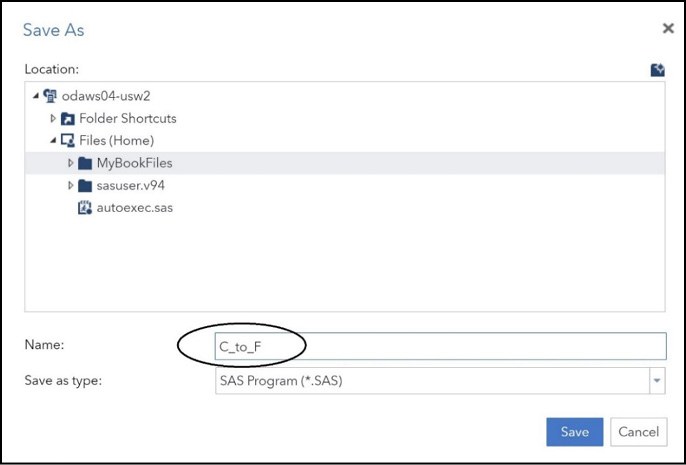
First, click the MyBookFiles folder. Next enter the program name (in this example, it is C_to_F.sas) and click Save. You can name your SAS program anything you like (as long as it meets the naming conventions for files on your computer). The extension .SAS is automatically added to the file name.
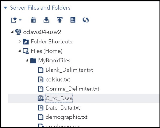
If you look in the Navigation Pane, you will now see the program C_to_F.sas in the list (Figure 7.12).
Figure 7.12: Contents of the MyBookFiles Folder
SAS programs can read just about any type of text data, whether it consists of numbers and letters, separated by delimiters (such as a CSV file), or whether the data values are arranged in fixed columns. This section just scratches the surface of the incredible versatility of this statement.
Let’s start out by reading a file where data values (either character or numeric) are separated by delimiters. The following file, called demographic.txt (stored in the MyBookFile folder), contains the following data values:
Variables in the File demographic.txt
ID
Gender (M or F)
Age
Height (in inches)
Weight (in pounds)
Party (political party affiliation (I=Independent, R=Republican, D=Democrat))
Here is the file.
File 7.2: demographic.txt
012345 F 45 65 155 I
131313 M 28 70 220 R
987654 F 35 68 180 R
555555 M 64 72 165 D
172727 F 29 62 102 I
You want to create a SAS data set called Demo from this raw data file. Proceed as follows:
Program 7.2: Reading Text Data from an External File
data Demo;
   infile “~/MyBookFiles/demographic.txt”;
   input ID $ Gender $ Age Height Weight Party $;
run;
You simply list the variable names in the same order as the data values in the file. As you can probably guess, a dollar sign ($) following a variable name indicates that you want to read and store this value as character data. Notice that ID is being stored as a character value so that any leading zeros will be maintained. This is a good time to mention that SAS has only two variable types: character and numeric. By default, all numeric values are stored in 8 bytes (64 bits). In most programs, you specify the length of character variables. In this first program, because no character variable lengths are specified, a default length of 8 bytes (characters) is used to store each of the character values (even though Gender and Party are only one character in length). You will see several methods of determining the storage length for character data later in this book.
Here is the SAS log that is produced when you run this program.
Figure 7.13: The SAS Log from Program 7.2
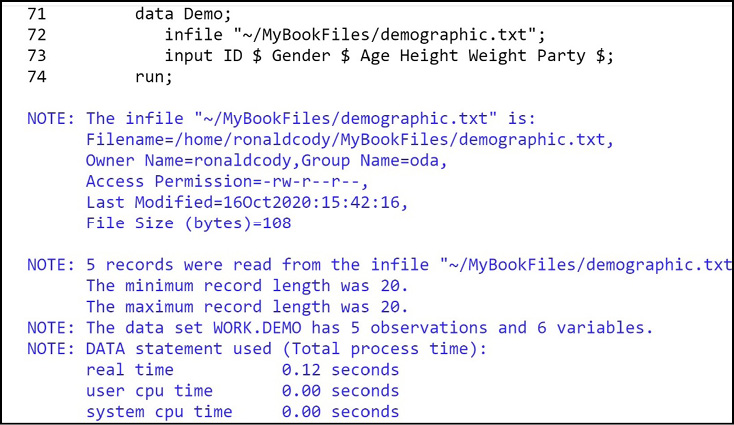
You see information about the input data file and note that 5 records were read (as expected) and the fact that a SAS data set, WORK.DEMO, was created. Unless you specify a storage location for your SAS data set, SAS places it in the WORK library. Data sets in the WORK library are temporary and disappear when you close your SAS session. You will see how to read and write permanent SAS data sets in Chapter 9. In the SAS log, you also see information about the real and CPU time used.
If you click the OUTPUT DATA tab, you will a list of variables and your data like this:
Figure 7.14: Contents in the OUTPUT DATA Tab
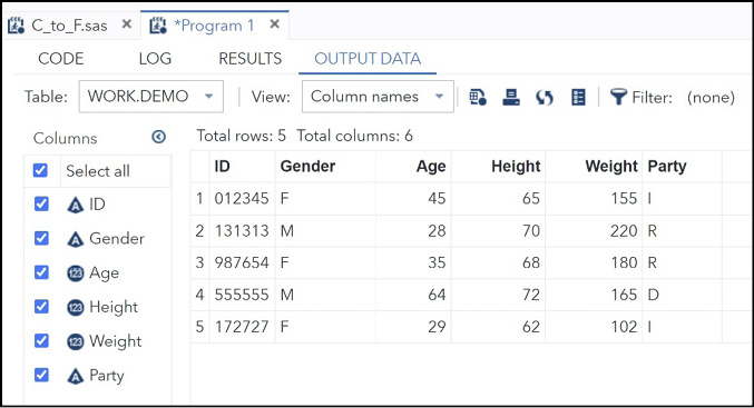
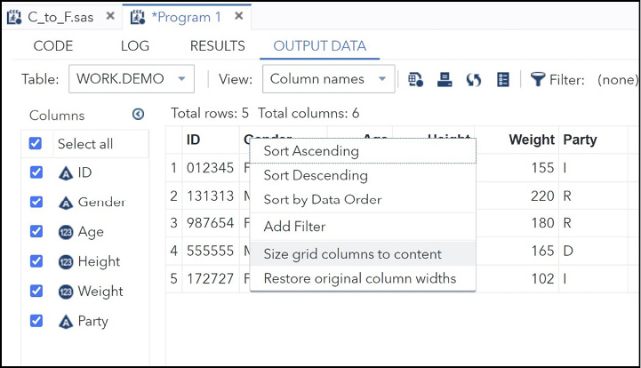
To adjust the column widths in this display, this author first right-clicked on one of the columns in the top row of the table and selected the option “Size grid columns to content”. (See Figure 7.15.)
As you saw in the first part of this book, you can now use the TASKS tab to summarize the data or produce plots. However, because this is the programming section of the book, let’s use PROC FREQ to compute frequencies and demonstrate how procedure options and statement options affect the results.
Program 7.3: Computing Frequencies from the Demo Data Set
data Demo;
   infile “~/MyBookFiles/demographic.txt”;
   input ID $ Gender $ Age Height Weight Party $;
run;

title “Computing Frequencies from the Demo Data Set”;

proc freq data=Demo;
   tables Gender Party;
run;
You use PROC FREQ to compute frequencies on any of your variables. Use a TABLES statement to specify which variables you want to include in your results. These can include both character and numeric variables. If you include any numeric variables in the list, PROC FREQ will compute the frequency on every unique value—it does not group values into bins (there are other procedures that can produce histograms). If you do not use a TABLES statement, PROC FREQ will compute frequencies on all the variables in your data set.
The output from Program 7.3 is shown below.
Figure 7.16: Output from Program 7.3
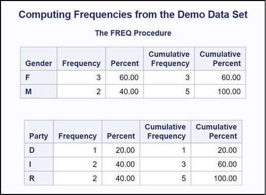
In the frequency tables, you see frequency, percent, cumulative frequency, and cumulative percent for the two variables Gender and Party. The output you see results from the default settings for this procedure. In most cases, you will want to include procedure and statement options to control the output.
Most SAS procedures have what are called procedure options. These options affect how the procedure works, and they are placed between the procedure name and the semicolon. One popular procedure option used with PROC FREQ is ORDER=. There are several values that you can select for this option. For this example, if you use ORDER=FREQ, the frequencies are ordered from the most frequent to the least frequent.
You will most likely use procedure statements with most procedures as well. The TABLES statement in Program 7.3 is an example of a procedure statement. You can also add statement options to control how a statement works. The rule is that statement options are placed after a slash (/) following the statement. The TABLES option NOCUM (no cumulative statistics) is used in the next program to demonstrate a statement option. Let’s also see how the procedure option ORDER=FREQ and the statement option NOCUM affect the output.
Program 7.4: Adding Options to PROC FREQ
title “Adding Procedure Options and Statements”;
Proc freq order=freq;
   tables Gender Party / nocum;
run;
Your output now looks like this.
Figure 7.17: Output from Program 7.4
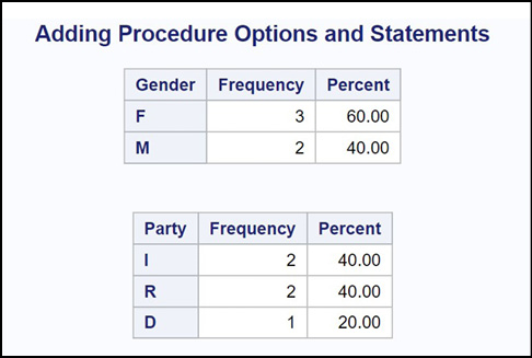
The tables are now displayed in decreasing frequency order (notice the change in the order of Party), and cumulative statistics are no longer included in the tables. In most cases, you will want to include the NOCUM option on your TABLES statement.
How SAS Works: A Look Inside the “Black Box”
Although you can write basic SAS programs without understanding what goes on inside the “black box,” a more complete understanding of how SAS works will make you a better programmer. Furthermore, this knowledge is essential when you are writing more advanced programs.
SAS processes the DATA step in two stages: In the first stage, called the compile stage, several activities take place. The SAS complier reads each line of code from left to right, top to bottom. Each statement is broken up into tokens, with certain keywords such as DATA and RUN causing certain actions to take place. What is important to you as a programmer, is to know that this is the stage where the data descriptor for each of your variables is written out. The first time SAS encounters a variable in a DATA step, it decides whether that variable is numeric or character. If it is numeric, SAS gives it a default length of 8 bytes. If it is character, it has rules that it uses to determine the storage length. SAS character values can be a maximum of 32,767 bytes in length. In this first stage, your source code is also compiled into machine language. Also, during the compile stage, SAS determines which variables will be written out to the new data set and which variables will be dropped (i.e., not written out). One way of determining whether a variable is kept or dropped is by explicitly writing a KEEP or DROP statement in the DATA step or by including a KEEP= or DROP= data set option (more on that later).
In the second stage, called the execute stage, the program performs its functions of reading data, performing logical actions, iterating loops, and so on. When you are reading raw data from a file or if you have variables defined in assignment statements (such as the variable Temp_F in Program 7.1), SAS initializes each of these variables with a missing value at the top of the DATA step. During execution of the DATA step, these variables are usually given values, either from the raw data or from a computation. At the bottom of the DATA step (defined by the RUN statement), SAS performs an automatic output to one or more data sets. The DATA step continues its internal loop, reading data, performing calculations, and outputting observations to a data set. If you are reading data from a text file or from a SAS data set, the DATA step stops when you reach the end-of-file marker on any file.
At this point, you understand how to write a simple program using the SAS OnDemand for Academics. You understand the various windows inside SAS Studio. You can read external data where blanks are used as delimiters and produce simple reports. The next chapter explores the INPUT statement, one of the most powerful statements in SAS.