Chapter Ten: Development of post-disturbance vegetation in prairie wetlands

Arnold G. van der Valk    ^{Iowa State University, Ames, IA, United States}

Abstract

It has long been recognized that plants are adapted to specific environmental conditions (e.g., soil moisture, soil chemistry, air temperature, and light levels) and that the distribution of plants varies along environmental gradients producing coenoclines (community gradients found along environmental gradients). Freshwater wetlands such as prairie potholes are ideal systems for studying coenoclines because their coenoclines are short and the main factor controlling the distribution of species along them is water depth. These wetlands undergo oscillatory waterlevel fluctuations that can at times result in destruction of most of their vegetation. Such disturbances provide an opportunity to study the development of post-disturbance coenoclines. This chapter reviews what is known about post-disturbance coenocline development in prairie wetlands, addresses the development of new coenoclines when pre- and post-disturbance water levels are the same or different, and reports on some models of coenocline development.

Keywords

Coenoclines; Wet-dry cycles; Dry marsh; MERP; Reflooding

Introduction

Why does a particular plant species or assemblage of plant species grow in a given place at a given time? In some cases, the answer to this question may be self-evident, for example, the species composition of a crop field in Iowa on July 1, 2005. In other cases, an answer may be beyond our grasp for the time being because of the complexity of the vegetation and absence of essential studies of its development, for example, a particular patch of lowland tropical rainforest in the Amazon basin on July 1, 2005. It has long been recognized (Cittadino, 1990) that plants are adapted to specific environmental conditions (e.g., soil moisture, soil chemistry, air temperature, and light levels) and that the distribution of plants varies along environmental gradients (McIntosh, 1967; Whittaker, 1967). Early on, consequently, plant ecologists believed that it should be possible to predict the distribution of species along environmental gradients on the basis of their physiological tolerances. The distribution of plant species along coenoclines (i.e., community gradients found along environmental gradients), however, is not necessarily solely a function of the physiological tolerances of adult plants. Plant species first have to reach a suitable site and become established for them to be found along a particular coenocline. In other words, seed dispersal patterns and seed germination requirements can also play a role in the distribution of plants along environmental gradients (van der Valk, 1992).

Plant ecologists have taken three different approaches to understanding and, ultimately, to predicting the distribution of species along coenoclines: (1) conducting observational studies of the distribution of species along environmental gradients; (2) doing experimental studies of coenocline development; and (3) developing mathematical models of coenocline development. Studies of coenocline development are still rare because it is often difficult to manipulate environmental conditions along coenoclines. Freshwater wetlands make an ideal system for studying coenoclines because their coenoclines are often very short and the main factor controlling the distribution of species along them is usually water depth (Spence, 1982). Water depths often change cyclically in wetlands (e.g., in North American prairie wetlands), and water depths can be manipulated in wetlands.

Prairie wetlands are found in the northcentral part of North America (van der Valk, 1989, 2005a). Major observational studies of the vegetation dynamics of prairie wetlands can be found in Walker (1959, 1965), Weller and Spatcher (1965), Millar (1973), Weller and Fredrickson (1974), van der Valk and Davis (1978), Shay and Shay (1986), Kantrud et al. (1989a, b), Shay et al. (1999), Swanson et al. (2003), Euliss Jr. et al. (2004), and van der Valk (2005a). Reviews of observational studies are found in Kantrud et al. (1989a, b) and Euliss Jr. et al. (2004). Information on water level fluctuations in prairie wetlands can be found in Euliss Jr. and Mushet (1996), LaBaugh et al. (1987, 1998), Woo and Rowsell (1993), Winter and Rosenberry (1995, 1998), Winter (1989, 2003), van der Kamp and Hayashi (1998), van der Kamp et al. (1999, 2003), Johnson et al. (2004), van der Valk (2005b), and Chapter 9 by Hayashi and van der Kamp.

In the prairie pothole region, changes in total annual precipitation result in oscillatory waterlevel fluctuations (van der Valk, 2005b). There are a variety of possible responses to these water level fluctuations along coenoclines in prairie wetlands (Euliss Jr. et al., 2004; van der Valk, 2005b). The cyclical elimination and re-establishment of emergent vegetation caused by water levels described by Weller and Spatcher (1965) and van der Valk and Davis (1978) are features only of deeper and usually larger prairie wetlands. These vegetation cycles, locally called wet-dry cycles, typically have a period of 10 to 20 years. In these wetlands, high water levels periodically extirpate all or most of their emergent vegetation, and it becomes re-established during subsequent periods when standing water is absent or very shallow (drawdowns). In other words, because high water results in the destruction of most of their vegetation, these wetlands undergo periodic disturbances (sensu Grime, 1979). Unlike most other kinds of disturbances (e.g., fire), which are very intense, brief phenomena, periods of high water have to last for years for them to destroy the vegetation; even then, only a subset of the species, primarily emergent species, may be killed.

These periodic disturbances provide an opportunity to study how species become re-established along elevation gradients when water levels drop, that is, coenocline development. Prairie wetlands are a good model system for studying the development of post-disturbance coenoclines. One, they are herbaceous wetlands whose species reach maturity in 1 to 3 years. Two, the entire flora of these wetlands is present in their seed bank, which eliminates dispersal uncertainties. Three, because they contain a variety of emergent vegetation types along an elevation (water depth) gradient, it is feasible to study the development of an entire coenocline, not just one vegetation type. Four, it is possible to manipulate their water levels and to do controlled studies of the destruction and redevelopment of their coenoclines.

In this chapter, I review what is known about post-disturbance coenocline development in prairie wetlands. I emphasize identifying factors (e.g., seed germination, seedling survival, water depth tolerances) that control the establishment and distribution of species along an elevation gradient. Over the last 40 years, the effects of water level changes on the coenoclines in prairie wetlands have been investigated by using observational studies, experimental studies, and models. The results of experimental and modeling studies will be emphasized in this chapter, especially those from a 10-year experimental study of water level changes, the Marsh Ecology Research Program (MERP), carried out in an experimental complex in the Delta Marsh, Manitoba, Canada (Murkin et al., 2000). After some brief background information about wet-dry cycles and MERP, I address three topics: (1) the development of a new coenocline when pre- and post-disturbance water levels are the same; (2) the development of new coenoclines when post-disturbance water levels differ from pre-disturbance water levels; and (3) the latest models of coenocline development.

Wet-dry cycles

The various stages during wet-dry cycles caused by water level fluctuations were first described by Weller and Spatcher (1965). They outlined a five-stage cycle: dry marsh (drawdown), dense marsh (mostly emergent cover), hemimarsh (50% emergent, 50% open water), open marsh (more than 50% open water), and open water marsh (emergents largely or completely eliminated). The open water marsh persists until the next drought, which lowers water levels, eventually exposing the marsh sediments. This marks the start of the next dry marsh stage. Later studies of these wet-dry cycles by van der Valk and Davis (1976, 1978) established the central role of seed banks (viable seed in the sediments) for the persistence of plant species in these wetlands and the importance of the dry marsh stage for the re-establishment of emergent species. Fig. 10.1, which is taken from van der Valk and Davis (1978), outlines the vegetation cycle that occurs in deeper and larger prairie potholes [i.e., classes IV and V of Stewart and Kantrud, 1971, 1972], in which a significant range of water levels (ca. 1.5 to 2 m) can occur. In their version of the wet-dry cycle, van der Valk and Davis (1978) modified the cycle proposed by Weller and Spatcher (1965) by combining the hemimarsh and open marsh stages, during both of which emergent vegetation is declining. The four stages in the van der Valk and Davis cycle (Fig. 10.1) are the dry marsh, regenerating marsh (= dense marsh), degenerating marsh (= hemimarsh and open marsh), and lake marsh (= open water marsh). It is the re-development of the emergent sections of coenoclines initiated during the dry marsh stage and the fate of the species along them during the regenerating marsh stage that is the focus of this chapter.

Fig. 10.1 Idealized wet-dry cycle in a semi-permanent prairie pothole. (From van der Valk, A. G., Davis, C. B., 1978. The role of the seed bank in the vegetation dynamics of prairie glacial marshes. Ecology 59, 322–335).

Marsh ecology research program

Wet-dry cycles are not confined to palustrine wetlands but also occur in prairie lacustrine wetlands. Walker (1959, 1965) studied vegetation changes caused by water level fluctuations in the Delta Marsh at the south end of Lake Manitoba, Manitoba, Canada. The range of water levels observed in the Delta Marsh historically was about 1.5 m, which is similar to that observed in deeper palustrine prairie-pothole wetlands. In the early 1960s, water level control structures were built around Lake Manitoba to prevent flooding of farms and villages near the lake during wet years. This significantly reduced the range of water level fluctuations in the Delta Marsh and changed its flora and fauna; most notably it caused a large decline in the number of waterfowl nesting in the marsh (Batt, 2000). Concerns about the condition of the Delta Marsh because of the stabilization of its water levels prompted the organization of Marsh Ecology Research Program (MERP).

As part of MERP, 10 experimental wetlands were constructed in 1979 by partitioning off a portion of Delta Marsh into 10 contiguous, rectangular cells, each between 5.5 and 7 ha in area (Fig. 10.2). Beginning in 1980, water levels were manipulated in these cells for the next 10 years to simulate a wet-dry cycle. There were three water level treatments (Fig. 10.3): normal, medium, and high. During the first year or two of MERP, water levels in the cells were maintained at the stabilized water level in the Delta Marsh (247.5 m); this is called the baseline period. (All water levels are elevations above mean sea level.) This was followed by 2 years of high water (248.5 m), the deep flooding period, and 1 or 2 years of low water (247.0 m), the drawdown period. During the drawdown years, the cells were free of standing water. Because the length of the drawdown had little impact on coenocline development, it is ignored in this chapter. During the last 5 years, the reflooding period, water levels were maintained at 247.5 m in the normal treatment, at 247.80 m in the medium, and at 248.1 m in the high treatment. There were four replicates of normal and three replicates of medium and high treatments. More detailed descriptions of MERP and the MERP cells can be found in Murkin et al. (2000).

Fig. 10.2 Location of the Marsh Ecology Research Program study site in the Delta Marsh, Manitoba, Canada. (From Murkin, H. R., van der Valk, A. G., Clark, W. R., (Eds.), 2000. Prairie Wetland Ecology: The Contribution of the Marsh Ecology Research Program. Iowa State University Press, Ames, IA).

Fig. 10.3 The MERP water level treatments. In the normal-1 treatment, cells were drawn down (247 m) for only 1 year (1984), while in the normal-2, medium, and high treatments, cells were drawn down for 2 years (1983 and 1984). The baseline year when all cells were at 247.5 m was 1980. Each cell was deep flooded (248.5 m) for 2 years beginning in 1981 or 1982. The three reflooding treatments, normal (247.5 m), medium (247.8 m), and high (248.1 m), began in 1985 and ended in 1989.

The coenocline that was found in the cells at the beginning of MERP consisted primarily of four monodominant emergent zones and a submersed aquatic zone (Fig. 10.4). Scolochloa festucacea (Willd.) Link and Phragmites australis (Cav.) Trin. zones covered most of the upper sections of the gradient. The lower sections were dominated by Typha glauca Godr. and Scirpus lacustris L. spp. glaucus (Sm.) Hartm. The submersed zone at the lowest elevations was dominated by a mixture of Potamogeton spp., especially P. pectinatus L., Utricularia vulgaris L., Myriophylum spicatum L., Najas flexilis (Willd.) Rostk. & Schmidt, Ceratophyllum demersum L. Plant nomenclature is based on Scoggan (1978–1979).

Fig. 10.4 Idealized coenocline in the Marsh Ecology Research Program cells in the Delta Marsh, Manitoba, Canada. (From Batt, B. D. J., 2000. The Delta marsh. In: Prairie Wetland Ecology. (Murkin, H. R., van der Valk, A. G., and Clark, W. R., Eds.), pp. 17–33. The Contribution of the Marsh Ecology Research Program, Iowa State University Press, Ames, IA).

Among the coenocline-related studies conducted as part of MERP were a detailed examination of the seed banks of the MERP complex before the start of water level treatments (Pederson, 1981; Pederson and van der Valk, 1985), field studies of recruitment during the drawdown years (van der Valk, 1986; Welling et al., 1988a, b), field studies of the fates of emergent species when the cells were flooded (Meredino and Smith, 1991; van der Valk, 1994, 2000; van der Valk et al., 1994), experimental studies of recruitment from seed banks (van der Valk and Pederson, 1989; Meredino et al., 1990; Meredino and Smith, 1991), seed germination studies of the dominant species (Galinato and van der Valk, 1986), and water-depth tolerance studies of the dominant emergent species (Squires and van der Valk, 1992). In addition, two new models were developed to predict the distribution of emergent species along coenoclines in the MERP cells (de Swart et al., 1994; van der Valk, 2000; Seabloom et al., 2001).

Coenocline development: Same pre- and post-disturbance water levels

During the drawdown period (Fig. 10.3), new coenoclines began to develop in the MERP cells (Welling et al., 1988a, b; van der Valk and Welling, 1988). Several factors or some combination of them (Fig. 10.5) could be responsible for the final distribution of emergent species along these new coenoclines, including the following:

1. 1. Composition of seed bank along the elevation gradient
2. 2. Differential seed germination along the elevation gradient
3. 3. Differential seedling survival along the elevation gradient during the drawdown
4. 4. Differential adult survival along the elevation gradient after reflooding, and
5. 5. Exploitative competition

Fig. 10.5 The major factors that may affect the distribution of species along a post-disturbance coenocline. (From van der Valk, A. G., Welling, C. H., 1988. The development of zonation in freshwater wetlands: an experimental approach. In: Diversity and Pattern in Plant Communities. (During, H. J., Werger, M. J. A., and Willems, J. H., Eds.) pp. 145–158. SPB Academic Publishing, The Hague, The Netherlands).

The relative abundances (i.e., percentage of the total number of seeds, seedlings, or adults in a given elevation range out of the total number found over the entire elevation gradient) of Scolochloa festucacea, Phragmites australis, Typha glauca, and Scirpus lacustris as seeds, seedlings, and adults along coenoclines in the MERP cells are presented in Tables 10.1 to 10.4. Only data for the normal treatment in the reflooding years is presented in these tables. The baseline data illustrate the pre-disturbance distribution of adults of these species along the elevation gradient and the seedbank data the pre-disturbance distribution of their seeds. The drawdown and reflooding data illustrate the post-disturbance distributions of their seedlings and adults.

Table 10.1

Relative (%) abundance of Scolochloa festucacea in the marsh ecology research program cells during the baseline year, in the seed bank, during the first and second years of the drawdown, and during the 5 reflooding years^a.

Elevation (m)	Baseline	Seedbank	Drawdown 1	Drawdown 2	Reflooding 1	Reflooding 2	Reflooding 3	Reflooding 4	Reflooding 5
248	0	8	1	4	0	0	0	0	0
247.9	2	3	0	1	0	0	0	0	0
247.8	14	5	15	3	0	1	5	9	5
247.7	40	13	37	25	5	16	37	34	50
247.6	37	25	19	23	22	47	44	54	44
247.5	8	34	25	23	41	15	9	3	1
247.4	0	10	3	19	26	13	4	0	0
247.3	0	0	0	0	2	2	1	0	0
247.2	0	0	0	3	2	0	0	0	0
247.1	0	0	0	0	3	6	0	0	0

a Relative abundance is based on areal cover during the baseline years and relative number of seeds, seedling, or shoots per unit area during all other years. The elevations with the highest relative abundances are given in bold. Only data for the cells in the normal treatment are presented for the reflooding years.

Table 10.2

Relative (%) abundance of Phragmites australis in the marsh ecology research program cells during the baseline year, in the seed bank, during the first and second years of the drawdown, and during the 5 reflooding years^a.

Elevation (m)	Baseline	Seedbank	Drawdown 1	Drawdown 2	Reflooding 1	Reflooding 2	Reflooding 3	Reflooding 4	Reflooding 5
248	16	20	0	0	0	0	0	0	0
247.9	23	20	0	0	0	0	0	0	0
247.8	21	9	12	0	0	0	0	0	0
247.7	16	8	8	20	0	0	8	11	19
247.6	14	11	12	1	0	0	2	1	2
247.5	6	20	23	3	38	40	34	40	40
247.4	2	6	30	60	48	42	34	40	33
247.3	0	2	15	13	1	5	11	8	4
247.2	0	1	0	3	12	14	11	1	2
247.1	0	3	0	0	0	0	0	0	0

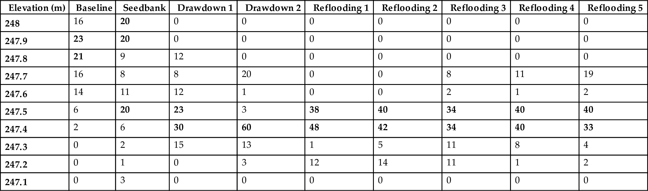
a Relative abundance is based on areal cover during the baseline years and relative number of seeds, seedling, or shoots per unit area during all other years. The elevations with the highest relative abundances are given in bold. Only data for the cells in the normal treatment are presented for the reflooding years.

Table 10.3

Relative (%) abundance of Typha glauca in the marsh ecology research program cells during the baseline year, in the seed bank, during the first and second years of the drawdown, and during the 5 reflooding years^a.

Elevation (m)	Baseline	Seedbank	Drawdown 1	Drawdown 2	Reflooding 1	Reflooding 2	Reflodding 3	Reflooding 4	Reflooding 5
248	0	4	0	0	0	0	0	0	0
247.9	0	3	0	0	0	0	0	0	0
247.8	1	8	0	0	0	0	0	0	0
247.7	7	6	2	1	0	1	1	2	2
247.6	19	17	0	2	0	0	8	6	5
247.5	31	19	9	6	6	6	23	19	23
247.4	24	33	7	8	14	9	7	10	13
247.3	14	8	77	13	36	50	36	44	31
247.2	3	1	4	65	43	34	25	20	27
247.1	0	2	0	5	0	0	0	0	0

a Relative abundance is based on areal cover during the baseline years and relative number of seeds, seedling, or shoots per unit area during all other years. The elevations with the highest relative abundances are given in bold. Only data for the cells in the normal treatment are presented for the reflooding years.

Table 10.4

Relative (%) abundance of Scirpus lacustris in the marsh ecology research program cells during the baseline year, in the seed bank, during the first and second years of the drawdown, and during the 5 reflooding years^a.

Elevation (m)	Baseline	Seedbank	Drawdown 1	Drawdown 2	Reflooding 1	Reflooding 2	Reflooding 3	Reflooding 4	Reflooding 5
247.9	0	0	0	1	0	0	0	0	0
247.8	0	1	3	0	0	0	0	0	0
247.7	0	3	7	0	0	0	0	1	1
247.6	2	12	1	1	0	0	0	0	0
247.5	15	48	8	4	3	4	14	28	38
247.4	34	18	66	21	34	27	28	50	50
247.3	32	8	13	24	21	21	25	8	0
247.2	15	7	2	43	36	38	23	12	7
247.1	2	3	0	6	8	11	10	1	3

a Relative abundance is based on areal cover during the baseline years and relative number of seeds, seedling, or shoots per unit area during all other years. The elevations with the highest relative abundances are given in bold. Only data for the cells in the normal treatment are presented for the reflooding years.

Seeds of the four dominant emergents were found over a wider elevation range than adults of the same species. Seed densities were highest for most species at 247.5 m, the water's edge. Secondary dispersal by wind and water currents had a significant impact on the distribution of seeds of all species along the coenocline in the Delta Marsh (Pederson and van der Valk, 1985). During the baseline period, adult populations were most abundant at higher elevations (Phragmites australis and Scolochloa festucacea) or lower elevations (Scirpus lacustris) than their seeds in the seed bank. Because the pre-disturbance distribution of their seeds was over a wider range than the post-disturbance distribution of adult plants, seed distribution per se did not affect the final distribution of the dominant emergent species along post-disturbance coenoclines.

The elevations at which seedlings of emergent species were most abundant during the first year of the drawdown were either higher (e.g., Scolochloa festucacea) or lower (e.g., Typha glauca) than the elevations at which their seeds were most abundant. The largest discrepancy between seed and seedling distribution patterns was for Phragmites australis. The seeds of P. australis had a bimodal distribution, with maxima at 247.9 to 248.0 m and at 247.5 m. No seedlings of Phragmites were found during the drawdown years (or subsequently) at the higher elevations (Table 10.2). Seedling densities were much lower for Scirpus lacustris, Scolochloa festucacea, and Typha glauca during the second year of the drawdown (van der Valk and Welling, 1988). The net effect of this decline was that maximum seedling densities for most species were found at lower elevations during the second year of the drawdown. This shift resulted in Phragmites australis seedlings being most abundant at 247.4 m, an elevation at which very few adult plants were found in the pre-disturbance coenocline. Overall, the percentage overlap of adult distributions during the baseline years and seedlings during the second year of the drawdown were 59% for Scolochloa, 22% for Phragmites, 38% for Typha, and 67% for Scirpus. In other words, although all four dominant species were found along both the pre- and post-disturbance coenoclines, their initial post-disturbance distributions, especially those of Phragmites and Typha, were different from those on the pre-disturbance coenocline. This difference was primarily caused by seedling establishment (germination, survival) patterns.

Studies of the effect of environmental conditions on seed germination from the seed bank in the Delta Marsh (van der Valk and Pederson, 1989; Meredino et al., 1990) and in other prairie wetlands (Seabloom et al., 1998) have shown that seedling establishment is highly dependent on environmental conditions during drawdowns (Table 10.5), especially soil moisture, soil salinity, and soil temperature. Differences in soil moisture can alter not only seedling densities but also the species composition of the vegetation that develops during drawdowns (van der Valk and Pederson, 1989). Likewise, seedling survival is highly dependent on adequate soil moisture. The percentage germination of seeds of emergent species was not uniform over the entire elevation range over which they were found (van der Valk and Welling, 1988).

Table 10.5

Number of seedlings recruited from seed bank samples from the delta marsh in drawdowns that began in May, June, July, and August 1988.

Species	May	June	July	August
Scolochloa festucacea	10	39	58	0
Phragmites australis	16	21	11	0
Typha glauca	140	495	311	18
Scirpus lacustris	300	218	130	0

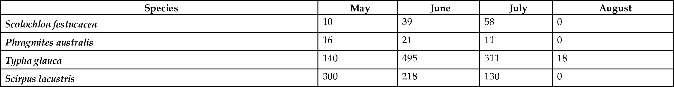
Adapted from Meredino, M. T., Smith, L. M., Murkin, H. R., Pederson, R. L., 1990. The response of prairie wetland vegetation to seasonality of drawdown. Wildl. Soc. Bull. 18, 245–251.

During the reflooding years in the normal treatment cells when these cells were flooded again to 247.5 m, the distribution of three species, Scolochloa, Typha, and Scirpus, gradually became more similar to their distribution along the pre-disturbance coenocline. By the fifth year of the reflooding period (Table 10.1), the percentage overlap in the distribution of Scolochloa with that during the baseline years was 89%. For Typha (Table 10.3) and Scirpus (Table 10.4), their overlap was 60%. The water depth tolerances of the adults eventually resulted in the post-disturbance coenocline coming to resemble the pre-disturbance coenocline more closely. For Phragmites, however, the overlap was only 27%. The post-disturbance coenocline also differs from the pre-disturbance coenocline in that Typha had its highest relative abundance at the lowest elevations, not Scirpus lacustris. Even after 7 years (Fig. 10.6), the distribution of emergent species along the post-disturbance coenocline was not identical to that along the pre-disturbance coenocline.

Fig. 10.6 Relative abundance of Scolochloa festucea, Phragmites australis, Typha glauca, and Scirpus lacustris along the elevation gradient in the Marsh Ecology Research Program cells during the pre-disturbance (baseline) and post-disturbance (5th year of reflooding) coenoclines.

Why was the post-dispersal coenocline different from the pre-disturbance coenocline? Although all four emergent species became re-established along the post-dispersal coenoclines, they did not become re-established initially within the elevation ranges at which they occurred in the pre-disturbance coenoclines. After establishment, these species were not able to adjust their distributions. The only changes that occurred during the five reflooding years along the elevation gradient were that emergent species declined in abundance in areas too deep for them to persist and expanded clonally in areas with more optimal water depths. They never moved up- or down-slope into more optimal water depths as is generally predicted to occur. There were two major reasons for their inability to adjust their distributions. One, the seeds of these four emergent species do not normally germinate under water (van der Valk, 1981), and two, there was no indication that the seeds of any emergent germinated in the field during the reflooding years in the MERP cells. Thus, these species could not become established at the higher or lower elevations by recruitment from the seed bank. Initially, the clonal spread of these species at elevations at which they became established was restricted to areas that were free of other emergent species. It was only in the last few years of the reflooding period, when species growing at water levels that they could not tolerate began to die, that any significant expansion of emergent species upslope (Phragmites, Table 10.2) or downslope (Typha, Table 10.3) occurred. In summary, recruitment patterns of emergent species along newly forming coenoclines had lasting effects, and the distribution of species along coenoclines was not simply a function of their water depth tolerances.

Coenocline development: Different pre- and post-disturbance water levels

In prairie wetlands, post-disturbance water levels may not necessarily return to pre-disturbance water levels. Water levels in wetlands are also sometimes permanently altered to improve the wetland as waterfowl or fish habitat, to reduce flooding in adjacent areas, to reduce the area of unwanted wetland species, and for many other reasons. It is often assumed that raising or lowering water levels will cause the various vegetation zones (i.e., the entire coenocline) in a wetland to shift up- or downslope (van der Valk, 1994). However, there is evidence that wetland coenoclines may not respond in the same way to raising water levels as to lowering them (Bukata et al., 1988). In other words, wetland coenoclines can shift downslope when water levels are permanently lowered (Fig. 10.7), but may not be able to shift upslope when water levels are permanently raised (Fig. 10.8). When water levels are lowered, coenoclines can shift downslope largely because the emergent species can move downslope either clonally or by becoming established from seed at lower elevations that are not flooded. As  seen in the MERP cells in which water levels were returned to pre-disturbance levels, emergent species cannot become established from seed at flooded higher elevations and they seem to have only a limited ability to shift their position through clonal growth.

Fig. 10.7 Effect of permanently lowering mean interannual (x_i) water level on a wetland coenocline: (A) the original coenocline, (B) the first year or two after water levels are lowered, (C) the coenocline under the new water-level regime. (From van der Valk, A.G., 1991. Response of wetland vegetation to a change in water level. In: Finlayson, C.M., Larsson, T. (Eds.), Wetland Management and Restoration. 3992 Swedish Environmental Protection Agency report).

Fig. 10.8 Effect of permanently raising mean interannual (x_i) water level on a wetland coenocline: (A) the original coenocline, (B) the first year or two after water levels are raised, (C) the coenocline under the new water-level regime. (From van der Valk, A.G., 1991. Response of wetland vegetation to a change in water level. In: Finlayson, C.M., Larsson, T. (Eds.), Wetland Management and Restoration. 3992 Swedish Environmental Protection Agency report).

When water levels are permanently raised, coenoclines have been predicted to respond in two ways (van der Valk, 1994): (1) the entire coenocline shifts upslope (the migration model) and (2) the coenocline is significantly altered in composition (the extirpation model). The latter model implies little or no shift in the location of species along the elevation gradient except their extirpation at elevations at which they cannot tolerate the water depth. Specifically, the extirpation model predicts that some species may be eliminated or significantly reduced in abundance and that the post-disturbance coenocline will be compressed or shortened when compared to the pre-disturbance coenocline. There were no barriers within or at the upper ends of the cells that would prevent emergent species from moving into more optimal water depths upslope. In other words, there were no dikes at the upper ends of these cells.

In the medium and high treatments of MERP, post-disturbance water levels were raised permanently by 30 and 60 cm, respectively, above the pre-disturbance water level of 247.5 m. Because the cells in the medium and high treatment experienced the same deep flooding period (disturbance) that eliminated emergents and the same drawdown period, the initial post-disturbance coenoclines in cells in these treatments were identical to those previously described in the normal treatment.

An experimental study of the water depth tolerances of the dominant emergent species in the Delta Marsh (Squires and van der Valk, 1992) indicated that these emergents fell into two fairly distinct groups. Some species (Scirpus lacustris ssp. glaucus and Typha glauca) grew best in deep water (ca. + 45 cm), while others (Scolochloa festucacea, Phragmites australis, and Scirpus lacustris ssp. validus (Vahl) T. Koyama) grew best in shallow water (+ 20 cm or less). This pattern is consistent with their distribution in the MERP cells during the baseline period (Tables 10.1–10.4) when only Scirpus lacustris ssp. glaucus was present in the cells. To illustrate the response of shallow and deep water species to the medium and high treatments, Tables 10.6 and 10.7 give the mean water depth and frequency of occurrence of Scolochloa, a shallow water species, and Typha, a deep water species, in all three treatments during the reflooding period (1985–1989).

Table 10.6

Mean water depth and frequency of Scolochloa festucacea in the normal, medium, and high water-level treatments from 1985 to 1989^a.

Treatment	Year
	1985	1986	1987	1988	1989	Mean
Mean water depth (m)
Normal	− 0.02	0.01	− 0.05	− 0.08	− 0.06	− 0.04
Medium	0.15	0.23	0.08	0.04	0.06	0.11
High	0.49	0.45	0.20b	0.09b	0.19b	0.33
Frequencyc
Normal	149	246	212	169	151	185
Medium	186	240	77	73	62	128
High	115	155	48b	30b	20b	74

a A negative number indicates that the species was growing at an elevation above 247.5 m.

^b Species absent from one or more cells in 1987, 1988, and 1989.

^c These are absolute frequencies (i.e., the number of times a species was recorded on a grid sampling of vegetation maps of the relevant cells in a given year. See de Swart et al. (1994) for details.

Table 10.7

Mean water depth and frequency of Typha glauca in the normal, medium, and high water-level treatments from 1985 to 1989.

Treatment	Year
	1985	1986	1987	1988	1989	Mean
Mean water depth (m)
Normal	0.13	0.10	0.07	0.07	0.10	0.09
Medium	0.25	0.34	0.27	0.25	0.25	0.27
High	0.44	0.57	0.52	0.51	0.42	0.49
Frequencya
Normal	23	137	146	186	194	137
Medium	66	152	119	123	117	115
High	104	191	129	130	181	147

a These are absolute frequencies (i.e., the number of times a species was recorded on a grid sampling of vegetation maps of the relevant cells in a given year. See de Swart et al. (1994) for details.

In the medium and high treatments, as in the normal treatment, Scolochloa was more abundant in 1986 than 1985. In 1987, however, Scolochloa frequency declined in all three treatments; this decline continued through 1989. In the medium and high treatments, Scolochloa frequency in 1987 was nearly 70% lower than in 1986, while in the normal treatment it declined only about 15% (Table 10.6). During 1985 and 1986, this species was able to survive in areas that were too deep for it to tolerate permanently by mobilizing stored reserves of carbohydrates from rhizomes. These reserves were exhausted by 1987. The decline of Scolochloa festucacea, Scirpus lacustris ssp. validus, and other shallow water species after several years of high water has also been recorded in other studies (Millar, 1973; Neckles, 1984) and is consistent with experimental studies of water-depth tolerances of these emergents (Neil, 1990, 1993; Waters and Shay, 1990; Squires and van der Valk, 1992). Because of the disappearance of Scolochloa from deeper parts of the cells, the mean water depth at which it was found declined after 1986 (Table 10.6). Its mean water depth in the medium treatment was 0.15 m in 1985 and 0.06 m in 1989 while in the high treatment it went from 0.49 m to 0.19 m.

Typha glauca (Table 10.7) also increased in frequency from 1985 to 1986. It was eliminated from some areas with very deep water in 1987, but only in the medium and high treatments did its frequency decline by about 20% and 30%, respectively, in 1987. Its frequency increased again in 1988 and 1989 because of its clonal spread, mostly into areas where shallow water species had been eliminated. The mean water depth at which Typha was found in any treatment, however, changed little from 1985 to 1989. In the medium treatment, it was 0.25 m in 1985 and 1989; in the high treatment, it was 0.44 m in 1985 and 0.42 m in 1989 (Table 10.7).

By 1989, the coenoclines in the medium and high treatments were significantly different from those in the normal treatment (Fig. 10.9). Scirpus lacustris was undetectable in the medium and high treatments in 1989. The other three emergents were growing in deeper water and were less frequent than in the normal treatment. By 1989, between 35% and 45% of the emergent vegetation in the medium and high treatment cells had been eliminated (van der Valk et al., 1994). Although some emergent losses (ca. 5%) were caused by herbivory by muskrats (Clark and Kroeker, 1993; Clark, 2000), most were caused by the loss of two species (Scolochloa festucacea [Table 10.6] and Scirpus lacustris ssp. validus and glaucus). The emergent sections of the coenocline in the normal treatment in 1989 covered an elevation range of 70 cm while those in the medium and high treatments covered a range of 60 cm and 40 cm, respectively (Fig. 10.9). During the baseline period, it covered a maximum range of 90 cm in the MERP cells. Assuming an equal slope, the coenoclines in the medium and high treatments were shorter than those in the normal treatment and during the baseline period. In summary, the medium and high treatment coenoclines had fewer species, lower species frequencies, and smaller elevation ranges than the coenoclines in the normal treatment and during the baseline period.

Fig. 10.9 Mean relative abundance of emergent species along post-disturbance coenoclines in the Marsh Ecology Research Program cells in the normal, medium, and high water treatments during the fifth year of the reflooding period (1989).

Species growing along the new coenoclines in the medium and high treatment were unable to shift their positions along the water depth gradient. In areas too deep to support their growth, emergent species were extirpated. Emergents did spread by clonal growth into areas with water depths that they could tolerate, especially after emergents previously growing in these areas had disappeared. All the data from the MERP study support the extirpation model (Fig. 10.8).

Models of coenocline development

The first conceptual model of wet-dry cycles was published by van der Valk (1981). This simple model, based primarily on plant life history characteristics (seed dispersal syndromes, seed germination requirements, and life expectancy), could only predict changes in the overall composition of a wetland's flora during various stages of wet-dry cycles (Fig. 10.1). For emergent species, as noted, both seed germination and life expectancy are highly dependent on water depth, with the absence of standing water, a drawdown, being a particularly crucial time for the recruitment of emergent species. Because it was not a spatially explicit model, it could not predict the distribution of species along coenoclines.

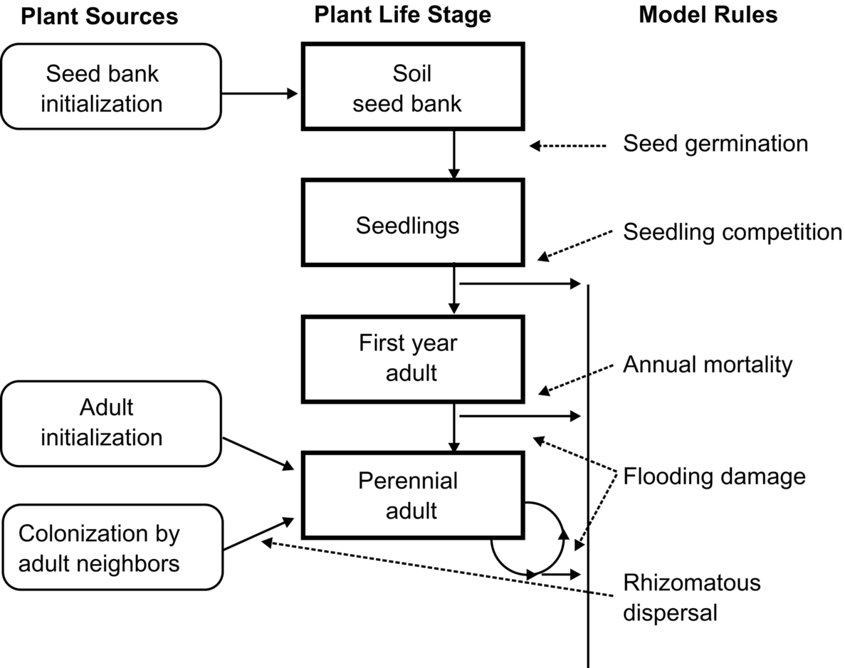
During MERP, two models of coenocline development were constructed and tested. The simpler of these models is the niche model of de Swart et al. (1994). The niche model assumes that water depth alone is sufficient to predict the distribution of emergent species along coenoclines in the MERP cells. The niche model uses logistic regression equations developed from data on the distribution of emergent species along elevation gradients during the pre-disturbance (baseline) years to predict the probability of finding a given emergent species at a given location in the MERP cells in the post-disturbance years. The second model is the spatially explicit model of Seabloom et al. (2001). In this cellular automaton model, the cells of the MERP complex are divided into 3 m by 3 m units. In each unit, emergent species can exist in four stages: dormant seeds, seedlings, first-year adults, and mature adults with clonal growth. Five sets of rules determine the probability that a given species would go from one stage to another in a unit (Fig. 10.10). Mature adults of only a single species can persist in a unit. A species can become dominant in a unit because it was the dominant species at the start of a simulation run, it colonized an empty adjacent unit, or it germinated from the seed bank and survived as a seedling and first-year adult in the unit (Fig. 10.10). These and other rules incorporated into the spatially explicit models were derived from a variety of studies of vegetation dynamics in prairie wetlands, not from the MERP studies.

Fig. 10.10 The structure of the spatially explicit model of coenocline development. (From Seabloom, E. W., Moloney, K. A., van der Valk, A. G., 2001. Constraints on the establishment of plants along a fluctuating water-depth gradient. Ecology 82, 2216–2232).

Both the niche and spatially explicit models were used to generate vegetation maps of the MERP cells by predicting the dominant emergent species in each 3 m by 3 m unit in each cell. The elevation of each unit was derived from a detailed topographic map of each MERP cell. This enabled the water depth of every unit in each cell in each year to be estimated. For more model details and procedures used to test these models, see de Swart et al. (1994) and Seabloom et al. (2001). The simulated vegetation maps generated by each model were compared to actual vegetation maps derived from low-level aerial photographs. Both the simulated maps and actual vegetation maps had the same resolution (3 m by 3 m).

Fig. 10.11 shows the mean proportion of the MERP cells predicted by both models to be covered with each emergent species and the actual proportions of each species estimated from aerial photographs. The accuracy of both models was high during periods when the cells were flooded, but low during the drawdown period (Fig. 10.11). During the reflooding period (1985 through 1989), the accuracy of both models increased with time. The niche model was the least accurate during the drawdown period because it greatly overestimated the amount of Phragmites australis. It was also unable to predict the presence of species that had not been part of the pre-disturbance coenocline. Because it does not incorporate time lags, the niche model also did more poorly predicting the abundance of emergent species during the first couple of years of the reflooding period (Fig. 10.11).

Fig. 10.11 Proportion of the Marsh Ecology Research Program cells covered by dominant emergent species and mudflat annuals predicted by the niche and spatially explicit models and the actual proportions estimated from aerial photographs. Scirpus acutus = Scirpus lacustris ssp. glaucus. (From Seabloom, E. W., Moloney, K. A., van der Valk, A. G., 2001. Constraints on the establishment of plants along a fluctuating water-depth gradient. Ecology 82, 2216–2232).

An examination of the model results confirms that constraints on species' ability to colonize areas creates both short- and long-term deviations from predicted distribution patterns based solely on water depth. Species were constrained because of seedling recruitment patterns, because they could not move upslope in response to an increase in water level, and because of landscape geometry in some cases. In prairie wetlands with their wet-dry cycles, the composition of coenoclines cannot necessarily be accurately predicted solely from local water depths at any given time. In the MERP cells, recruitment constraints were minimal because all the emergent species were present in the seed bank. This eliminated dispersal problems that could affect the initial composition of the coenocline during a drawdown, and thus establishment effects caused by preemption (i.e., the order in which species arrived at a site). Consequently, dispersal and establishment constraints will be much more important in the development of most other coenoclines. For example, in recently restored prairie potholes in which there is no seed bank of any consequence (Wienhold and van der Valk, 1989), the development of coenoclines is highly dependent on seed dispersal from other sites. Consequently, coenoclines vary widely among restored wetlands (Galatowitsch and van der Valk, 1996; Seabloom and van der Valk, 2003).

Neither the niche nor the spatially explicit model incorporated herbivory, plant pathogens, exploitative competition, or many other factors known to influence zonation patterns in wetlands (Spence, 1982). These did not have a detectable role in the development of the new coenoclines in the MERP cells. For example, muskrats, whose feeding and lodge building activities can have a significant impact on the abundance and distribution of emergents in some prairie wetlands (Weller and Spatcher, 1965), were never common in the MERP cells (Clark, 2000). In wetlands subject to less frequent and extreme water level fluctuations, including other kinds of prairie wetlands (Euliss Jr. et al., 2004), these other factors may play a role in coenocline development.

Conclusions

The almost complete destruction of coenoclines in some prairie wetlands occurs periodically because of several years of above-normal water levels. Post-disturbance coenoclines, however, are not necessarily identical to pre-disturbance coenoclines, even when water levels under which the post-dispersal coenoclines develop are identical to those during the pre-disturbance period. Although pre- and post-disturbance coenoclines had the same species composition, the elevation ranges over which emergent species were found along these coenoclines were not similar. Differences in initial patterns of seed germination and seedling survival that resulted in the development of the pre-disturbance and post-disturbance coenocline seem to be responsible for these distribution differences. Thus, differences in soil moisture and temperature during the early stages of coenocline development can have lasting effects. When post-disturbance water levels are higher than pre-disturbance water levels, post-disturbance coenoclines are very different from pre-disturbance coenoclines. Emergent species were not able to shift their location upslope. Instead, they died out in areas too deep for them. This effectively compresses the coenoclines by eliminating emergents at their deep ends and even resulted in the extirpation of species along some post-disturbance coenoclines. Spatially explicit models of coenocline development confirmed the  lasting impacts of constraints on post-disturbance coenocline development.

Disturbances over time result in changes in the plant communities found along environmental gradients. These changes can be very minor when pre- and post-disturbance environmental conditions are similar and much greater when pre- and post-disturbance environmental conditions are dissimilar. In the Delta Marsh, field observations and other data (e.g., aerial photographs) document vegetation changes over three wet-dry cycles. The post-disturbance vegetation that developed during the drawdown and regenerating stages of these cycles was in all three cases different from the pre-disturbance vegetation. Recruitment of species along newly developing coenoclines in the Delta Marsh is from the seedbank. Because dispersal uncertainties were not a factor, the results of the MERP study should not be extrapolated to situations where post-disturbance dispersal of species is required for coenocline development. In such cases (e.g., recently restored prairie wetlands), coenocline composition and structure are highly variable from wetland to wetland.

References

Batt B.D.J. The Delta marsh. In: Murkin H.R., van der Valk A.G., Clark W.R., eds. Prairie Wetland Ecology. Ames, IA: Iowa State University Press; 2000:17–33 The Contribution of the Marsh Ecology Research Program.

Bukata R.P., Bruton J.E., Jerome J.J., Harris W.S. An evaluation of the impact of persistent water level changes on the areal extent of Georgian Bay/North Channel marshland. Environ. Manag. 1988;12:359–368.

Cittadino E. Nature as the Laboratory: Darwinian Plant Ecology in the German Empire, 1880–1900. Cambridge, UK: Cambridge University Press; 1990.

Clark W.R. Ecology of muskrats in prairie wetlands. In: Murkin H.R., van der Valk A.G., Clark W.R., eds. Prairie Wetland Ecology. Ames, IA: Iowa State University Press; 2000:287–313 The Contribution of the Marsh Ecology Research Program.

Clark W.R., Kroeker D.W. Population dynamics of muskrats in experimental marshes at Delta, Manitoba. Can. J. Zool. 1993;71:1620–1628.

de Swart E.O.A.M., van der Valk A.G., Koehler K.J., Barendregt A. Experimental evaluation of realized niche models for predicting responses of plant species to a change in environmental conditions. J. Veg. Sci. 1994;5:541–552.

Euliss Jr. N.H., Mushet D.M. Water-level fluctuation in wetlands as a function of landscape condition in the prairie pothole region. Wetlands. 1996;16:587–593.

Euliss Jr. N.H., Labaugh J.W., Fredrickson L.H., Mushet D.M., Laubhan M.K., Swanson G.A., Winter T.C., Rosenberry D.O., Nelson R.D. The wetland continuum: a conceptual framework for interpreting biological studies. Wetlands. 2004;24:448–458.

Galatowitsch S.M., van der Valk A.G. Characteristics of recently restored wetlands in the prairie pothole region. Wetlands. 1996;16:75–83.

Galinato M.I., van der Valk A.G. Seed germination traits of annuals and emergents recruited during drawdowns in the Delta Marsh, Manitoba, Canada. Aquat. Bot. 1986;26:89–102.

Grime J.P. Plant Strategies and Vegetation Processes. Chichester, UK: Wiley; 1979.

Johnson W.C., Boettcher S.E., Poiani K.A., Guntenspergen G. Influence of weather extremes on the water levels of glaciated prairie wetlands. Wetlands. 2004;24:385–398.

Kantrud H.A., Krapu G.L., Swanson G.A. Prairie Basin Wetlands of the Dakotas: A Community Profile. Biological Report 85. Washington, DC: U.S. Fish and Wildlife Service; 1989a.

Kantrud H.A., Millar J.B., van der Valk A.G. Vegetation of wetlands of the prairie pothole region. In: Van der Valk A.G., ed. Northern Prairie Wetlands. Ames, IA: Iowa State University Press; 1989b:132–158.

LaBaugh J.W., Winter T.C., Adomaites V.A., Swanson G.A. Hydrology and chemistry of selected prairie wetlands in the cottonwood lake area, Stutsman County, North Dakota, 1979–1982. In: U.S. Geological Survey Professional Paper 1431, Denver, CO. 1987.

LaBaugh J.W., Winter T.C., Rosenberry D.O. Hydrologic functions of prairie wetlands. Great Plains Res. 1998;8:17–37.

McIntosh R.P. The continuum concept of vegetation. Bot. Rev. 1967;33:130–187.

Meredino M.T., Smith L.M. Influence of drawdown date and reflood depth on wetland vegetation establishment. Wildl. Soc. Bull. 1991;19:143–150.

Meredino M.T., Smith L.M., Murkin H.R., Pederson R.L. The response of prairie wetland vegetation to seasonality of drawdown. Wildl. Soc. Bull. 1990;18:245–251.

Millar J.B. Vegetation change in shallow marsh wetlands under improving moisture regime. Can. J. Bot. 1973;51:1443–1457.

Murkin H.R., van der Valk A.G., Clark W.R., eds. Prairie Wetland Ecology: The Contribution of the Marsh Ecology Research Program. Ames, IA: Iowa State University Press; 2000.

Neckles H.A. Plant and Macroinvertebrate Response to Water Regime in a Whitetop Marsh. M.S. Thesis St. Paul, MN: University of Minnesota; 1984.

Neil C. Effects of nutrients and water levels on species composition in prairie whitetop (Scolochloa festucacea) marshes. Can. J. Bot. 1990;68:1015–1020.

Neil C. Growth and resource allocation of whitetop (Scolochloa festucacea) along a water depth gradient. Aquat. Bot. 1993;46:235–246.

Pederson R.L. Seed bank characteristics of the Delta marsh, Manitoba: applications for wetland management. In: Richardson B., ed. Selected Proceedings of the Midwest Conference on Wetland Values and Management. Navarre, MN: Freshwater Society; 1981:61–69.

Pederson R.L., van der Valk A.G. Vegetation change and seed banks in marshes: ecological and management implications. In: Transactions of the Forty-Ninth North American Wildlife and Natural Resources Conference; 271–280. 1985;vol. 49.

Scoggan H.J. The Flora of Canada. Parts 1–4. Ottawa, Canada: National Museum of Natural Science; 1978–1979.

Seabloom E.W., van der Valk A.G. The development of vegetative zonation patterns in restored prairie pothole wetlands. J. Appl. Ecol. 2003;40:92–100.

Seabloom E.W., van der Valk A.G., Moloney K.A. The role of water depth and soil temperature in determining initial composition of prairie coenoclines. Plant Ecol. 1998;138:203–216.

Seabloom E.W., Moloney K.A., van der Valk A.G. Constraints on the establishment of plants along a fluctuating water-depth gradient. Ecology. 2001;82:2216–2232.

Shay J.M., Shay C.T. Prairie marshes in western Canada, with specific reference to the ecology of five emergent macrophytes. Can. J. Bot. 1986;64:443–454.

Shay J.M., de Geus P.M., Kapinga M.R.M. Changes in shoreline vegetation over a 50-year period in the Delta Marsh, Manitoba in response to water levels. Wetlands. 1999;19:413–425.

Spence D.H.N. The zonation of plants in freshwater lakes. Adv. Ecol. Res. 1982;12:37–125.

Squires L., van der Valk A.G. Water-depth tolerances of the dominant emergent macrophytes of the Delta marsh, Manitoba. Can. J. Bot. 1992;70:1860–1867.

Stewart R.E., Kantrud H.A. Classification of Natural Ponds in the Glaciated Prairie Region. Washington, DC: U.S. Fish and Wildlife Service Resource Publication No. 92; 1971.

Stewart R.E., Kantrud H.A. Vegetation of Prairie Potholes, North Dakota in Relation to Quality of Water and Other Environmental Factors. Washington, DC: U. S. Geological Survey Professional Paper 585-D; 1972.

Swanson G.A., Euliss Jr. N.H., Hanson B.A., Mushet D.M. Dynamics of a prairie pothole wetland complex: implications for wetland management. In: Winter T.C., ed. Hydrological, Chemical, and Biological Characteristics of a Prairie Pothole Wetland Complex Under Highly Variable Climate Conditions—The Cottonwood Lake Area, East-central North Dakota. 2003:55–94 U.S. Geological Survey Professional Paper 1675, Denver, CO.

van der Kamp G., Hayashi M. The groundwater recharge functions of prairie wetlands. Great Plains Res. 1998;8:39–56.

van der Kamp G., Stolte W.J., Clark R.G. Drying out of small prairie wetlands after conversion of their catchments from cultivation to permanent brome grass. J. Hydrol. Sci. 1999;44:387–397.

van der Kamp G., Hayashi M., Gallen D. Comparing the hydrology of a grassed and cultivated catchment in the semi-arid Canadian prairies. Hydrol. Process. 2003;17:559–575.

van der Valk A.G. Succession in wetlands: a Gleasonian approach. Ecology. 1981;62:688–696.

van der Valk A.G. The impact of litter and annual plants on recruitment from the seed bank of a lacustrine wetland. Aquat. Bot. 1986;24:13–26.

van der Valk A.G., ed. Northern Prairie Wetlands. Ames, IA: Iowa State University Press; 1989.

van der Valk A.G. Establishment, colonization and persistence. In: Glenn-Lewin D.C., Peet R.K., Veblen T.T., eds. Plant Succession: Theory and Prediction. London, UK: Chapman and Hall; 1992:60–102.

van der Valk A.G. Effects of prolonged flooding on the distribution and biomass of emergent species along a freshwater wetland coenocline. Vegetatio. 1994;110:185–196.

van der Valk A.G. Vegetation dynamics and models. In: Murkin H.R., van der Valk A.G., Clark W.R., eds. Prairie Wetland Ecology: The Contribution of the Marsh Ecology Research Program. Ames, IA: Iowa State University Press; 2000:125–161.

van der Valk A.G. The prairie pothole region of North America. In: Fraser L.H., Keddy P.A., eds. The World's Largest Wetlands: Ecology and Conservation. Cambridge, UK: Cambridge University Press; 2005a:393–423.

van der Valk A.G. Water-level fluctuations in North American prairie wetlands. Hydrobiologia. 2005b;539:171–188.

van der Valk A.G., Davis C.B. Seed banks of prairie glacial marshes. Can. J. Bot. 1976;54:1832–1838.

van der Valk A.G., Davis C.B. The role of the seed bank in the vegetation dynamics of prairie glacial marshes. Ecology. 1978;59:322–335.

van der Valk A.G., Pederson R.L. Seed banks and the management and restoration of natural vegetation. In: Leck M.A., Parker V.T., Simpson R.L., eds. Ecology of Soil Seed Banks. New York: Academic Press; 1989:329–346.

van der Valk A.G., Welling C.H. The development of zonation in freshwater wetlands: an experimental approach. In: During H.J., Werger M.J.A., Willems J.H., eds. Diversity and Pattern in Plant Communities. The Hague, The Netherlands: SPB Academic Publishing; 1988:145–158.

van der Valk A.G., Squires L., Welling C.H. An evaluation of three approaches for assessing the impacts of an increase in water level on wetland vegetation. Ecol. Appl. 1994;4:525–534.

Walker J.M. Vegetation Studies on the Delta Marsh. 1959 Manitoba, M.Sc. Thesis, University of Manitoba, Winnipeg, MB, Canada.

Walker J.M. Vegetation Changes with Falling Water in the Delta Marsh, Manitoba. Ph.D. Dissertation Winnipeg, MB, Canada: University of Manitoba; 1965.

Waters I., Shay J.M. A field study of the morphometric response of Typha glauca shoots to a water depth gradient. Can. J. Bot. 1990;68:2339–2343.

Weller M.W., Fredrickson L.H. Avian Ecology of a Managed Glacial Marsh. Living Bird; 269–291. 1974;12.

Weller M.W., Spatcher C.S. Role of Habitat in the Distribution and Abundance of Marsh Birds. Special Report 43 Ames, IA: Iowa Agriculture and Home Economics Experiment Station; 1965.

Welling C.H., Pederson R.L., van der Valk A.G. Recruitment from the seed bank and the development of zonation of emergent vegetation during a drawdown in a prairie wetland. J. Ecol. 1988a;76:483–496.

Welling C.H., Pederson R.L., van der Valk A.G. Temporal patterns in recruitment from the seed bank during drawdowns in a prairie wetland. J. Appl. Ecol. 1988b;25:999–1007.

Whittaker R.H. Gradient analysis of vegetation. Biol. Rev. 1967;42:197–264.

Wienhold C.E., van der Valk A.G. The impact of duration of drainage on the seed banks of northern prairie wetlands. Can. J. Bot. 1989;67:1878–1884.

Winter T.C. Hydrological studies of wetlands in the northern prairie. In: Van der Valk A.G., ed. Northern Prairie Wetlands. Ames, IA: Iowa State University Press; 1989:16–54.

Winter T.C. Geohydrological setting of the Cottonwood Lake Area. In: Winter T.C., ed. Hydrological, Chemical, and Biological Characteristics of a Prairie Pothole Wetland Complex Under Highly Variable Climate Conditions—The Cottonwood Lake Area, East-Central North Dakota. 2003:1–24 U.S. Geological Survey Professional Paper 1675, Denver, CO.

Winter T.C., Rosenberry D.O. The interaction of ground water with prairie pothole wetlands in the cottonwood Lake area, east-Central North Dakota, 1979–1990. Wetlands. 1995;15:193–211.

Winter T.C., Rosenberry D.O. Hydrology of prairie pothole wetlands during drought and deluge: a 17-year study of the cottonwood Lake wetland complex in North Dakota in the perspective of longer term measured and proxy hydrological records. Clim. Change. 1998;40:189–209.

Woo M.-K., Rowsell R.D. Hydrology of a prairie slough. J. Hydrol. 1993;146:175–207.