Chapter Eleven: Modeling fire effects on plants: From organs to ecosystems
Elizabeth J. Kleynhansa; Adam L. Atchleyb; Sean T. Michaletza a Department of Botany and Biodiversity Research Centre, University of British Columbia, Vancouver, BC, Canada
b Earth and Environmental Sciences, Los Alamos National Lab, Los Alamos, NM, United States
Abstract
Wildfires and prescribed burns have complex effects on vegetation and ecosystem function, ranging from minor injuries to tissue and organs to whole plant mortality and stand replacement. These effects are dependent on fire behavior characteristics and plant traits, but how they emerge from an interaction of fire behavior and plant physiology is not well understood. We propose a novel process-based modeling framework that links physics-based fire behavior models with trait-based plant physiological response models to investigate injury to the roots, stem and crown. Injuries are linked to whole-tree growth and mortality via xylem hydraulics and carbon budgets. Fire effects at higher levels of organization (populations to ecosystems) can be characterized by either performing spatially-explicit individual-based simulations or via metabolic scaling theory. Overall, our framework will be useful to scientists and managers alike to predict fire impacts across levels of biological organization.
Keywords
Wildfire; Prescribed burning; Fire behavior; Fire injury; Fire effects; Process-based models; Tree mortality
Acknowledgments
The authors acknowledge support from SERDP project RC18-1346.
Introduction
Wildland fires (including wildfire and prescribed burns) have many complex effects on vegetation and ecosystem function. These range from relatively minor injuries to tissues and organs (e.g., fire scars and crown scorch) to whole plant mortality and forest stand replacement. Fire effects are dependent upon fire behavior variables such as fire intensity and residence time, as well as plant traits such as bark thickness, stem diameter, tree height, and crown morphology (Bond and Keeley, 2005; Michaletz and Johnson, 2007; O'Brien et al., 2018; Bär et al., 2019; Scalon et al., 2020). Despite an increasing need to understand and predict fire effects in a changing climate (Flannigan et al., 2013), we still have only a limited understanding of how fire behavior variables interact with plant traits to affect plant functioning across levels of biological organization.
In this chapter, we outline the physical processes linking fire behavior, plant traits, and plant physiology to tree injuries and mortality, from individuals to ecosystems. We begin by reviewing the history of fire modeling, followed by background on combustion processes that influence fire behavior and spread, and a brief description of current approaches to modeling fire. We then describe ways in which trees are heated by fires, and how this leads to plant root, stem, and crown injuries. Injuries to plant roots, stems and crowns can then be used to determine the effects of fire on whole-plant functioning via changes in carbon and water budgets. Lastly, we describe how size-dependent mortality of individuals “scale up” to determine stocks and fluxes of ecosystems (e.g., total stand biomass, primary productivity, and evapotranspiration).
History of fire behavior and effects research
Fire ecology is concerned with the ecological patterns that emerge from a coupling of fire processes and ecological processes. Consequently, fire ecology research encompasses questions and approaches of two sub-disciplines: fire behavior and fire effects. Despite their shared interests and common goals, these sub-disciplines have developed in relative isolation of each other.
Fire behavior research began in the early 1900s, and after an initial descriptive phase, became dominated by engineers and physical scientists who introduced a process-based approach to the field (e.g., Hawley, 1926; Curry and Fons, 1940; Fons, 1946; Byram, 1959; Thomas, 1963). Fire effects research began around the same time (Clements, 1910), but grew out of the phytosociology and plant community ecology traditions and thus used a descriptive approach to characterize patterns of fire effects (e.g., Chapman, 1932; Heyward, 1939; Oosting, 1944; Curtis and Partch, 1948; Cottam, 1949). This led to the emergence of “the two solitudes” of fire ecology (Van Wagner, 1971), whereby fire behavior research considered the physical processes of fire and fire effects research focused on description of fire effects.
In the 1960s and 1970s, some researchers began using the process approach of fire behavior research to understand and explain the patterns described in fire effects research. Examples of this early work include the use of heat transfer theory to predict vascular cambium necrosis in tree stems (Spalt and Reifsnyder, 1962; Martin, 1963a; Reifsnyder et al., 1967; Gill, 1974) and the application of buoyant plume theory to predict the height of leaf necrosis in tree crowns (Van Wagner, 1973). Despite these efforts to marry the two lines of research, fire ecology generally continued to comprise two rather isolated research areas of fire behavior and fire effects (Butler and Dickinson, 2010; Dickinson and Ryan, 2010; Kavanagh et al., 2010; O'Brien et al., 2018).
What has limited the unification of fire behavior and fire effects research? One reason might be that, traditionally, linking process with pattern in fire ecology was difficult. As a consequence, fire effects research has focused on patterns of fire effects and not the mechanisms that cause them, while fire behavior research has focused on fire spread and not on the ecological processes that govern the availability and structure of vegetative fuels. Another reason is that the field was limited to relatively simple models of fire spread and buoyant plume behavior (reviewed in Weber, 1991; Mercer and Weber, 2001; Sullivan, 2009). This made it difficult to link fire behavior processes to the physiological and demographic processes that control fire effects. For example, early models such as those based on buoyant plume theory could successfully predict the height of leaf necrosis from low intensity fires with little to no wind (Van Wagner, 1973), but are less successful for predicting other injuries that depend on additional fire behavior variables beyond only buoyant plume temperature (e.g., radiation fluxes).
The approximations used in simpler mechanistic models (e.g., buoyant plume model) as well as non-mechanistic correlative models have resulted in these models being ineffective at representing heterogeneity in fire behavior. In contrast, more recent advances in process-based approaches such as computational fluid dynamics (CFD) models (reviewed below) allow us to now accurately resolve such heterogeneity at increasingly fine resolutions. CFD models can also characterize fire-atmosphere interactions (reviewed in Mell et al., 2009; Sullivan, 2009; Bakhshaii and Johnson, 2019) and three-dimensional forest fire spread at resolutions as fine as centimeters and spatial scales as large as hundreds of meters or kilometers (e.g., Linn and Cunningham, 2005; Mell et al., 2007, 2009). Nevertheless, these models are computationally expensive and thus, at present, cannot be used to model large high-intensity fires in real time.
To help build a more mechanistic and predictive fire ecology, current three-dimensional fire-atmosphere models must be coupled or linked to process models of fire effects on plants. This would be a major advance over earlier approaches that used relatively simple fire models that were generally steady-state, time-averaged approximations that could not be coupled to the fire effects in question. To lay the groundwork for such an approach, we next outline several key chemical and physical processes that are important for wildfire behavior and effects, before reviewing two CFD models that simulate these processes to make quantitative predictions of fire behavior in time and space.
Fundamentals of combustion and heat transfer
Physics-based three-dimensional fire spread models are derived from first principles of physics and chemistry. “Fire” is a combustion process whereby a positive feedback occurs between fuel supply rates and heat generated from combustion itself. In particular, volatile hydrocarbon fuels and oxygen mix causing an exothermic reaction that produces products such as carbon dioxide, water, carbon monoxide, and unburned carbon (i.e., soot and tar). The heat produced by combustion can be transferred to unburned fuel, driving additional oxidation reactions and causing the fire to spread. To gain more insight into these processes, we provide a brief overview below, although interested readers should refer to Holman (2002), Drysdale (2011) and Bergman and Lavine (2017) for more details.
Chemistry of combustion
Fire ignition requires a minimum amount of energy to initiate the oxidation of fuel. This minimum amount of energy is known as the activation energy Ea (J mol− 1), and it can be supplied through heat conduction, convection, and radiation. Following the activation of the chemical reaction, additional energy increases the reaction rate in an exponential fashion as described by the Arrhenius equation:
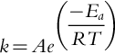
where R is the universal gas constant (8.314 J K− 1 mol− 1), T (K) is the absolute temperature of the reactants, k is the rate constant and A is the pre-exponential factor describing the frequency of collisions between particles in the correct orientation per second. The units of k and A are the same and depend on the order of the reaction; for example, a first order reaction will have units of s− 1 (Laidler, 1984; Firme, 2019).
Wildland fires consume both live and dead plant material. Plant cells predominantly consist of cellulose, but also contain hemicellulose, lignin, water, minerals, salts, extractables, and other inorganic compounds. For example, wood consists of approximately 41% to 53% cellulose, 15% to 25% hemicellulose and 16% to 33% lignin (Browning, 1963). These organic polymers exist in a solid state, so for the oxidation reactions of combustion to occur, the polymers must first be broken into shorter chains that can volatilize. This occurs via a thermal decomposition process called pyrolysis (Fig. 11.1).
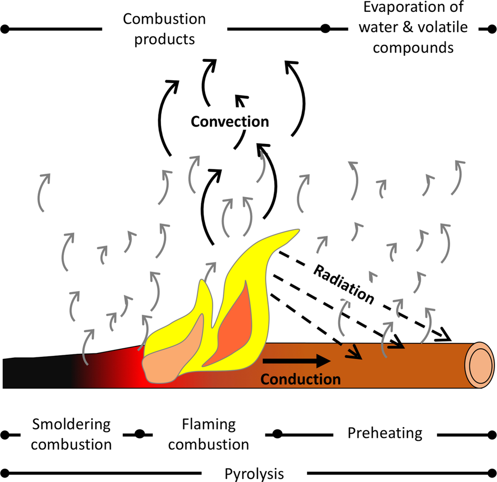
Three distinct stages of pyrolysis are helpful for understanding fire spread: preheating, flaming combustion, and smoldering combustion (Ward, 2001) (Fig. 11.1). During the preheating phase, unburned vegetation is subjected to radiation, convection (heating or cooling from air turbulence and flow), and conduction heat transfer. Preheating evaporates water and dries the fuel, and also decomposes organic polymers via pyrolysis reactions. Initially, pyrolysis is an endothermic reaction that requires energy to create volatile products and activate the reaction. However, once the rate of volatilization is sufficiently large and these products mix with oxygen in stoichiometric proportions, rapid oxidation reactions can occur, and an exothermic flame is produced (Fig. 11.1—flaming combustion). Such flames are known as “diffusion flames,” because fuel diffuses outward from a fuel rich interior of the flame, and oxygen diffuses inward from the exterior of the flame (Michaletz and Johnson, 2007). The rate at which the preheating phases take place determines the rate of fire spread. Furthermore, duration and depth of the flame can influence air entrainment, and thus wind can play an important role in influencing convective preheating and availability of oxygen to the fuel.
By-products of flaming combustion include char and ash, which build up on the surface of the fuel and slow the rate at which gaseous fuel and oxygen mix. When the rate of mixing is too slow to support flaming combustion, smoldering combustion commences (Fig. 11.1). Smoldering combustion lacks a flame and produces lower temperatures than flaming combustion (Ward, 2001; Michaletz and Johnson, 2007).
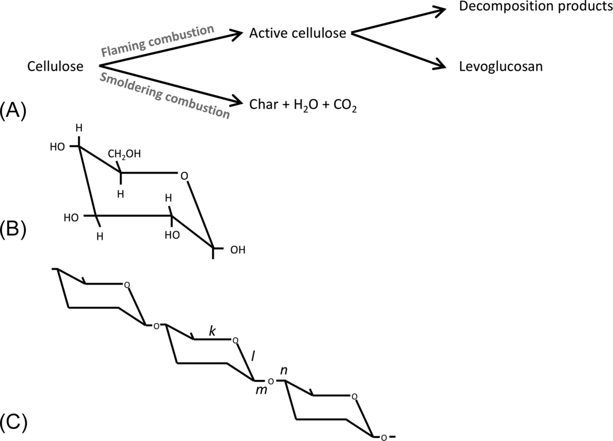
Flaming and smoldering combustion are associated with two distinct pathways of pyrolysis that involve different chemical reactions. For example, we consider two different pathways of cellulose degradation that occur in different thermal environments (Fig. 11.2A). When temperatures are low (200–280 °C) and/or moisture is present, cellulose degrades via char formation (Kilzer and Broido, 1965; Ward, 2001). This pathway is most typically associated with smoldering combustion and is often associated with the slow consumption of duff (Miyanishi, 2001) (Fig. 11.2A). Generally, it is thought that the bonds in position k or l break (Fig. 11.2C), so the polymer ring opens while the overall structure of the cellulose chain remains intact. The products of this reaction are char, H2O, CO, and CO2 (Drysdale, 2011). When temperatures are higher (280–340 °C), pyrolysis yields the volatile fuel levoglucosan (tar) which supports a gas-phase flame (Kilzer and Broido, 1965; Ward, 2001) (Fig. 11.2A and B). This fuel is highly unstable and readily oxidizes during combustion, releasing heat and other solid and gas phase products (Schindler and Hauser, 2004). Visually, bonds m or n are thought to break (Fig. 11.2C), causing the polymer chain to disintegrate and leaving the reactive ends exposed so that levoglucosan molecules can break away (Drysdale, 2011). This form of pyrolysis is associated with flaming combustion.
The chemical composition, water content, size, shape, and vertical and horizontal arrangement of fuel determines whether combustion reactions (char formation and volatilization) are self-sustaining, and how they will contribute to fire intensity and rate of spread. In the next section, we review heat transfer processes and their relevance to fire behavior and effects.
Physics of heat transfer
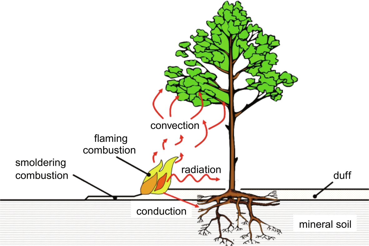
Heat released during combustion is transferred to unburned fuels through conduction, convection, and radiation (Fig. 11.3). Preheating of the fuel results in moisture loss, and may increase fuel temperatures to values that permit pyrolysis. Rates of preheating influence rates of fire spread. Because preheating involves conduction, convection and radiation, we describe each of these processes below (Drysdale, 2011; Michaletz, 2018).
Conduction
Conduction is the transfer of energy down a heat gradient within a (usually) solid medium, from hotter to colder areas. Higher-energy (warmer) molecules with greater random translational, internal rotational and vibrational motions collide with their neighbors, releasing energy. This energy is transferred from more energetic (warmer) to the less energetic (cooler) molecules, increasing the energy of less energetic molecules and causing them to similarly collide with their “down-stream” neighbors, yielding another energy transfer. In this way, energy is distributed across the medium without the bulk motion of the molecules (Michaletz and Johnson, 2007; Bergman and Lavine, 2017).
Fourier's law characterizes one-dimensional conduction heat transfer as
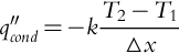
Here, the conduction heat flux qcond′′ (W m− 2) is proportional to the difference in temperature △ T between one location and another in the medium (i.e., T2 − T1) (K), the distance △ x (i.e., L1 − L2) (m) between the two locations, and the thermal conductivity k (W m− 1 K− 1) of the material. Different materials have different thermal conductivities as a result of differences in material density, temperature, and water content. For example, Martin (1963b, c) found that the thermal conductivities of wood and bark differ by about 20%, with bark having a lower thermal conductivity than wood. Lastly, the negative sign in Eq. (11.2) is present because heat transfer needs to be positive, and in this case the derivative or slope of heat transfer is negative (i.e., dT/dx = T2 − T1/L1 − L2) (Drysdale, 2011; Bergman and Lavine, 2017) (Fig. 11.4).
Convection
Convection is a process of heat transfer due to diffusion (random molecular motion) and the bulk motion of molecules (advection) such as the flow of air or water. Convection can either be free (natural) or forced.
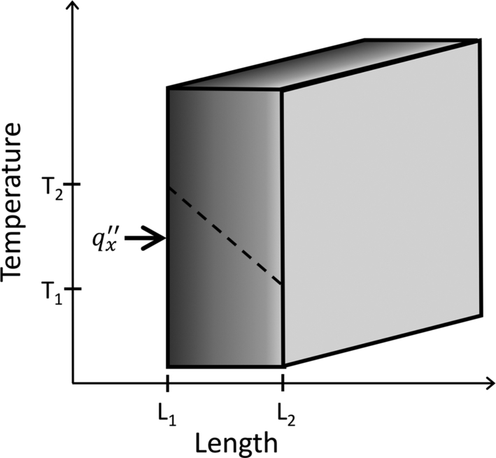
Free convection (Fig. 11.5A) occurs when the body-to-fluid temperature difference causes a gradient in fluid density. Gravity then acts upon these differences in density, yielding buoyancy forces that drive bulk movement of the fluid. The degree of the temperature gradient between the body and the fluid influences the rate of free convection. Higher rates of convection are obtained under larger temperature differences, and lower rates of convection are obtained under smaller temperature gradients (Michaletz and Johnson, 2007). In fires, the buoyant plumes rising above combusting fuels are a result of free convection (Fig. 11.3).
Forced convection occurs when fluid flowing over a body is driven by some external force, such as wind (Bergman and Lavine, 2017) (Fig. 11.5B). Consider a hot plate with temperature Ts subjected to a fluid with temperature T∞ under laminar flow conditions. Before the fluid reaches the plate (Fig. 11.5A), it has a uniform distribution of temperature and velocity (u∞). Once the fluid flows over the plate, a hydrodynamic (velocity) boundary layer develops, because the velocity of the moving particles at the plate-fluid interface is reduced to zero due to viscous forces. These particles reduce the velocity of the particles above them, and so on, so that the velocity of the fluid ranges from zero at the plate surface to u∞ in the free stream (Fig. 11.5B—velocity distribution). Similarly, due to the temperature difference between the plate and the fluid, a thermal boundary layer develops. For the thermal boundary layer, heat is transferred via conduction from the plate to stationary fluid particles at the plate-fluid interface, and via conduction and advection (bulk motion of the fluid) among fluid particles, creating a gradient in temperature away from the hot surface (Fig. 11.5A and B—temperature distribution). Boundary layers exist in both laminar and turbulent flow. Lastly, the depth of the velocity and temperature boundary layers need not be the same (Holman, 2002; Bergman and Lavine, 2017).
Heat transferred by convection is described by Newton's law of cooling, whereby the convection heat flux qconv′′ (W m− 2) is proportional to the convection heat transfer coefficient h (W m− 2 K− 1) and the body-to-fluid temperature difference △ T (Ts − T∞) (K), such that
The value of the convection heat transfer coefficient (h) depends on properties of both the solid surface (e.g., geometry and orientation) and the fluid (e.g., velocity, viscosity, and thermodynamic properties). For further details see Holman (2002) and Bergman and Lavine (2017).
Radiation
Unlike conduction and convection which both occur in a physical medium, radiation can occur in a vacuum because it transfers energy through electromagnetic waves or photons. Any matter that has a temperature greater than absolute zero emits thermal radiation. The amount of radiation emitted by a body (or emissive power) is determined by the amount of thermal energy stored in its surface and the rate at which this energy is released. This process is characterized by the Stefan-Boltzmann law, which quantifies the radiation heat flux (q′′radW m− 2) per unit time and area by a surface, such that
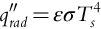
Here σ (5.669 × 10− 8 W m− 2 K− 4) is the Stefan-Boltzmann constant, Ts (K) is the surface temperature and ɛ (dimensionless) is the emissivity. When ɛ = 1, this equation describes the amount of energy emitted by an ideal radiator (i.e., a blackbody), but in reality most surfaces emit less energy, and this reduction relative to a blackbody is scaled through ɛ (where ɛ varies from 0 to 1) (Bergman and Lavine, 2017).
Radiation is an important mechanism of heat transfer for fires with a fuel bed diameter larger than about 0.3 m (Drysdale, 2011). Soot particles are the strongest source of thermal radiation from individual species within a fire, although electronic transitions of molecules also contribute (Sullivan, 2009; Blunck, 2018). Radiation contributes to fire spread by drying and preheating unburned fuel to the point of ignition. The proportion of radiation absorbed by unburned fuel depends on its absorptance, geometry, and orientation. For example, a body can only absorb radiation from another surface if it is in the “line of sight” of the emitting body, such as the sun warming you when you are standing outside in the open, but not when you are being shaded by a tree. Similarly, the angle of the surface relative to the emitter influences how much radiation is absorbed; for example, surfaces perpendicular to the sun's emitted radiation will absorb more energy than the same surface positioned at an angle to the emitted radiation. The influence of geometry, orientation, and distance on radiation flux between two surfaces can be quantified as a view factor (Howell, 1982), and this is needed to calculate how much radiation is transmitted between two bodies.
Modeling fire behavior
Combustion and heat transfer are at the heart of fire behavior, but these operate through a multitude of higher-level processes such as firebrand generation and transport (which can lead to the ignition of spot fires) or boundary layer dynamics and meteorology (e.g., wind, relative humidity, topographic effects). Combining all of these processes together to accurately simulate fire behavior and effects is extremely challenging. Nevertheless, over the last decades, important advances have been made that link fire processes across scales, from combustion chemistry to heat transfer physics to fire-atmosphere interactions.
Here we highlight two such models: FIRETEC (Linn, 1997; Linn et al., 2002) and Wildland-urban interface Fire Dynamics Simulator (WFDS) (Mell et al., 2007; McGrattan et al., 2013a, b). Both models are three-dimensional computational fluid dynamics (CFD) models that rely on partial differential equations to numerically solve for conservation of mass, momentum, energy, and chemical species. By solving for changes in variables such as temperature, velocity, and the mass fractions of gaseous species over time and space, these models can predict fire behavior, smoke generation, and smoke transport. Similarities in the approach to modeling fire of these two models include defining a domain volume based on the number of grid cells chosen, the approach to modeling turbulence, and how fuels are defined. For example, both models use a finite-volume, large eddy simulation (LES) approach to model turbulence, although WFDS also provides the option to simulate these dynamics through direct numerical simulation (Hoffman et al., 2016). Numerical grids are used to explicitly resolve large scale eddies and vortices, while small eddies and vortices are resolved with sub-grid scale models (Hoffman et al., 2016). Both models describe fuels as highly-porous, meaning that only thermally thin components of the vegetative fuel (e.g., leaves and thin branches) are assumed to combust and are modeled within the 3D numerical grids through mean and bulk quantities (e.g., moisture content, bulk density, surface area to volume ratios, etc.) (Hoffman et al., 2016). Although these models are similar in many respects, there are also important differences, the main one being that the energy equations are posed in terms of temperature for FIRETEC and enthalpy for WFDS (Hoffman et al., 2016). Nevertheless, both models predict rates of spread that agree with empirical data (Hoffman et al., 2016), suggesting they are suitable for simulating small fires of short duration (Bakhshaii and Johnson, 2019). More details of each model are provided below.
HIGRAD/FIRETEC
This modeling platform is based on the conservation of mass, momentum, and energy, and simulates fire-atmosphere interactions by linking the HIGRAD and FIRETEC models (Linn, 1997). HIGRAD (high gradient flow solver) is a CFD model that uses LES of the Navier-Stokes equations (Pimont et al., 2009) to simulate airflow over different terrains, vegetation types, and as a result of fire (Reisner et al., 1998). HIGRAD was developed to deal with abrupt changes in temperature and air flow gradients found in the vicinity of wildfires (Reisner et al., 1998, 2000). FIRETEC uses physics and chemistry to model combustion and heat transfer, and simulates aerodynamic drag and turbulence through LES (Pimont et al., 2009). FIRETEC is “self-determining,” meaning that the fire's behavior is predicted from dynamic physical processes that are dependent on both local and non-local processes (Linn et al., 2002). An example of a local process is preheated fuel that leads to faster ignition, while non-local processes include the effects of distant topography and coupled fire-atmosphere interactions that may alter the shape of the fireline. FIRETEC employs effective parameterizations at the grid cell scale where variables in the equations of conservation of mass, momentum, and energy are representative of the grid cell volume. As a result, rather than modeling the location of individual leaves and branches, or the sub-grid scale fluctuations in temperature due to flame dynamics, average fuel characteristics and temperature profiles are instead presented. Sub-grid scale processes, such as the rate of combustion reaction, are further represented by solving for turbulent kinetic energy within a cell based on pressure gradients of nearby cells (Pimont et al., 2009) and a probability distribution function of combustion as a function of cell temperature (Linn, 1997).
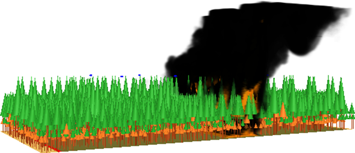
Wildland-urban interface Fire Dynamics Simulator (WFDS)
WFDS is a version of the NIST Fire Dynamics Simulator (FDS) for structural fires (McGrattan et al., 2013a, b) that has been extended to include fuels for vegetation (Mell et al., 2007, 2009). A visualization of a high intensity wildfire in a closed-canopy white spruce forest simulated by WFDS is shown in Fig. 11.6 (Michaletz et al., 2013). Like FIRETEC, WFDS is fully three-dimensional and uses a CFD approach to solve time-dependent equations describing the combustion, heat transfer, and motion of fluid. However, unlike FIRETEC, WFDS assumes that the chemical reaction between oxygen and gaseous fuel that results in combustion is independent of temperature, because mixing fuel and oxygen occurs over a much longer time scale than does heat generated during the chemical reaction (Bakhshaii and Johnson, 2019). To burn fuel, WFDS assumes a two-stage thermal decomposition process. Firstly, the fuel is assumed to dry out, then pyrolysis and char oxidation occur (Mell et al., 2009; Sullivan, 2009). Further details and comparisons between FIRETEC and WFDS can be found in Sullivan (2009), Hoffman et al. (2016), and Bakhshaii and Johnson (2019).
Fire effects on plants
Fire effects on plants have typically been divided into two types: first-order and second-order (Michaletz and Johnson, 2007; Hood et al., 2018; Bär et al., 2019). Generally, first-order effects are the direct effects of heating on plant tissues (e.g., fine root, cambium, phloem, bud, and foliage necrosis) that directly and significantly impair plant functioning and may ultimately lead to plant death. In comparison, second-order effects are indirect effects of first-order effects that may not immediately kill the plant, but may alter photosynthetic rates, water uptake, and/or increase susceptibility to insect and pathogen attack. Second-order effects may impair functioning and ultimately lead to death (Michaletz and Johnson, 2007; Hood et al., 2018; Bär et al., 2019). Below we describe the impact of fires on the different plant parts (roots, stem, and crown), and describe the models used to predict the injuries caused by heating. Although previous work has separated the discussion of first- and second-order effects (e.g., Michaletz and Johnson, 2007; Hood et al., 2018; Bär et al., 2019), we do not do that here since the separation is not clearly defined.
Heat is transferred to the roots, stem, and crown via radiation, conduction, and convection (Dickinson and Johnson, 2001; Michaletz and Johnson, 2007) (Fig. 11.3). The injuries sustained by a plant during a fire depend on a variety of factors, including the intensity and duration of heating (Bond and Keeley, 2005), plant growth rates and investment strategy (Hoffmann and Franco, 2003; Hoffmann et al., 2012), and functional traits such as bark thickness and bud size (Brando et al., 2012; Hoffmann et al., 2012; Scalon et al., 2020). Tissue necrosis results from protein denaturation and is usually assumed to occur at a threshold temperature of 60 °C (Hare, 1961; Rosenberg et al., 1971; Van Wagner, 1973). While this threshold temperature is widely used in fire effects models (e.g., Steward et al., 1990; Michaletz and Johnson, 2006b, 2008), rates of cellular injury increase exponentially with temperature so that tissue necrosis can result from long periods of heating at low temperatures or short periods of heating at high temperatures (Hare, 1961; Dickinson and Johnson, 2004).
Fire effects on roots
Root necrosis from fire depends on root traits such as diameter and depth (McLean, 1969; Smirnova et al., 2008), soil characteristics such as depth of organic layer, moisture content, and texture (Busse et al., 2010), and fire characteristics such as temperature and duration. Smoldering combustion generally causes more severe root injury than flaming combustion because, although it has lower temperatures, it occurs for a much longer duration and thus conducts heat to greater depths (Hartford and Frandsen, 1992; Michaletz and Johnson, 2007). For example, longleaf pine ecosystems with deep organic soil experienced smoldering combustion that led to substantial root necrosis (Varner et al., 2005, 2009; O'Brien et al., 2010). Similarly, Smirnova et al. (2008) found that deep smoldering adjacent to tree stems girdled coarse roots that were not insulated by mineral soil. This substantially injured the tree, since all of the roots below the girdle died as a result of carbon starvation.
Root injuries can result in depletion of root nonstructural carbohydrates (Varner et al., 2009) or reductions in whole-plant transpiration (O'Brien et al., 2010) and growth rates (Varner et al., 2009). They can also have long-term impacts on plants, since root necrosis results in a loss of stored resources and a reduced ability to acquire new resources. The reduction in stored and acquired resources results in a reduction in canopy conductance and carbon assimilation rates (O'Brien et al., 2010).
Root heating models
Several models consider soil heating by fire, enabling prediction of soil temperature profiles for various moisture contents (e.g., Steward et al., 1990; Campbell et al., 1994, 1995; Massman, 2015). None of these models, however, explicitly couple soil heating to root injuries. For example, Steward et al. (1990) assumed that root necrosis occurred when soil temperatures exceeded 60 °C, but they did not model heat conduction within the root. Large diameter roots in heated soils will have a temperature gradient from the exterior to the interior of the root (Michaletz and Johnson, 2007). This could be modeled by extending Chatziefstratiou et al.'s (2013) model of two-dimensional stem heating to roots. Since smoldering combustion generally results in heating of roots at low temperatures for extended periods of time, necrosis rates might be better characterized using a dose dependent response approach (e.g., Dickinson, 2002). For example, in a review of biological responses to soil heating, Pingree and Kobziar (2019) found that plant roots died within a range of temperatures between 48 °C and 65 °C when experiencing those temperatures for between 0.5 and 120 min. Moreover, Zeleznik and Dickmann (2004) observed substantial necrosis of red pine (Pinus resinosa) roots when they were exposed to temperatures of 52.5 °C for at least one minute.
In general, the effects of fire on roots is an area of study that requires more research. Especially needed are process-based models that investigate the impacts of fire on roots. A model such as this could help answer whether trees can die as a result of root necrosis alone. Hood et al. (2018) suggested that tree mortality due to root necrosis is unlikely because the mineral soil is a poor conductor of heat, and fires intense enough to kill roots will also significantly injure aboveground parts of the tree. But in a longleaf pine ecosystem that had experienced fire exclusion, Varner et al. (2005) suggested tree mortality was caused primarily by smoldering combustion of accumulated organic soil around the stem. While these contrasting effects are clearly the result of differences in fuels, fire behavior, and plant traits, they could all be predicted by properly parameterized process models.
Fire effects on stems
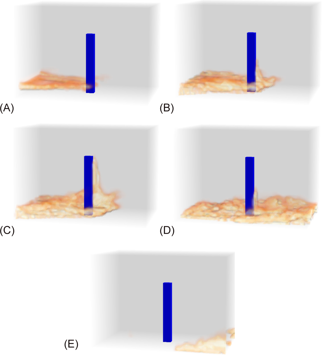
In general, tree stems experience uneven heating around their circumference during wildfires. The leeward side of the stem generally experiences flames with longer residence times and greater heights than the windward side, due to the interaction of flames with vortices in the turbulent leeward wake (Gill, 1974; Gutsell and Johnson, 1996). This results in differential heating around the stem, with greater heat fluxes and injuries on the leeward side (Gutsell and Johnson, 1996; Splawinski et al., 2019).
Fig. 11.7 illustrates the interaction between a moving fireline and the wake flow behind a tree stem. As the fire passes the stem, flames are drawn into the leeward wake (Fig. 11.7A), producing a standing leeward flame (Fig. 11.7B). As the fireline passes the stem, the height of the standing leeward flame increases (Fig. 11.7C) and then decreases (Fig. 11.7D). Once the trailing edge of the fireline moves past the vortices, the standing leeward flame has completely receded (Fig. 11.7E), but the sequence of events yielded an increase in flame residence time in the lee of the stem. Gutsell and Johnson (1996) estimated that this process increases the distance between the front and back of the fireline by two tree diameters.
The production of leeward vortices is governed by the stem diameter (d; m), the wind velocity (U; m s− 1), and the kinematic viscosity of air (v; m2 s− 1). Together, these variables comprise the Reynolds number (Re; dimensionless) which characterizes the boundary layer development and wake flow around a stem, such that

Laminar flow occurs for Re < 5, a pair of attached vortices exists for 5 ≤ Re < 40, and a wake of vortices (vortex street) occurs for Re ≥ 40 (see Gutsell and Johnson (1996) for more details). The magnitude of Re depends largely on stem diameter and wind speed; the effects of variation in kinematic viscosity with air temperature are small relative to those for tree size and wind speed, and can therefore generally be neglected. Re increases with stem diameter and wind speed, and these are key variables that determine the extent of stem and crown injury (Gutsell and Johnson, 1996; Dickinson and Johnson, 2001).
Plant stems are heated via radiation and convection from the fire (Fig. 11.3) (Dickinson and Johnson, 2001; Michaletz and Johnson, 2007). The amount of heat that is transferred into the stem depends on the fire residence time, the difference in temperature between the heated exterior and interior of the bole, the diameter of the tree, and various other traits such as bark thickness, bark moisture content, and wood density (van Mantgem and Schwartz, 2003; Brando et al., 2012; Wei et al., 2019).
Bark thickness has been found to be an excellent predictor of fire injuries (Dickinson and Johnson, 2004; Brando et al., 2012; Wei et al., 2019). In experimental fires in the Amazon, bark thickness explained 82% of the variation in rates of heat transfer through bark in more than 3000 stems from 24 tree species (Brando et al., 2012). Bark thickness varies within and between species, and tends to be linearly related to tree size, so that larger trees have thicker bark that provides more resistance to heat transfer (Spalt and Reifsnyder, 1962; Dickinson and Johnson, 2001; Brando et al., 2012). Similarly, the base of a stem has thicker bark than distal regions, so heating of phloem, cambium, and xylem requires longer residence times at the base of the stem (Glasby et al., 1987; Dickinson and Johnson, 2001).
The moisture contents and densities of bark and wood also influence fire effects on stems. The temperature of bark will be constrained to 100 °C until all of the moisture has evaporated; this “thermal arrest” means that bark with higher moisture content is more buffered against temperature extremes than bark with lower moisture content (Brando et al., 2012). Similarly, trees with denser wood are more fire resistant (Brando et al., 2012), probably because dense wood is more resistant to cavitation and deformation of xylem during fires (see below; Michaletz et al., 2012, Michaletz, 2018).
The composition of a tree stem is illustrated in Fig. 11.8. During a fire, heat conducts from the surface of the stem into the bark, phloem, cambium, and xylem. Due to the locations of these tissues, it was originally thought that tree mortality resulted from heat necrosis of phloem and cambium (Michaletz and Johnson, 2007); this is the cambium necrosis hypothesis (Michaletz et al., 2012, 2018). However, more recently it has been shown that tree mortality can also occur from cavitation and deformation of xylem (Balfour and Midgley, 2006; Kavanagh et al., 2010; Midgley et al., 2011; Michaletz et al., 2012; Bär et al., 2018); this is the xylem dysfunction hypothesis (Michaletz, 2018). These hypotheses are described in more detail in the following sections.
The cambium necrosis hypothesis
Post-fire plant mortality is often assumed to be a result of vascular cambium necrosis, because stem heating involves conduction through the bark, phloem, and cambium (Fig. 11.8). Phloem is the vascular tissue that transports carbon (photosynthates) from the leaves to basal parts of the plant, and vascular cambium is undifferentiated tissue responsible for secondary growth and repair of damaged phloem (Lalonde et al., 2004). Thus, heat necrosis of both phloem and cambium interrupts the downward translocation of carbon resources to the roots. If heating is extreme, phloem and cambium necrosis may occur around the entire circumference of the tree, resulting in girdling (Noel, 1970). Although girdled trees may survive for decades on nonstructural carbohydrates stored in the roots, they will ultimately die from hydraulic failure once the nonstructural carbohydrate reserves are depleted and fine root production can no longer occur (Michaletz et al., 2012; Michaletz, 2018; Bär et al., 2019).
Working under this cambium necrosis hypothesis, many models of post-fire tree mortality quantified heat conduction from the outside of a tree to the cambium (Peterson and Ryan, 1986; Costa et al., 1991; van Mantgem and Schwartz, 2003; Dickinson and Johnson, 2004; Dickinson et al., 2004; Jones et al., 2004, 2006; Butler and Dickinson, 2010). Several important insights have followed from these models, including the importance of including moisture in the thermal properties of bark and wood (Martin, 1963b, 1963c; Jones et al., 2004, 2006), that heating is not uniform around the circumference of the stem (Gill, 1974; Tunstall et al., 1976; Gutsell and Johnson, 1996), and thus that consideration of two-dimensional conduction is often necessary for accurately predicting heat transfer in tree stems (Chatziefstratiou et al., 2013).
The xylem dysfunction hypothesis
Although heat conducted into a stem will injure the phloem and cambium tissues first, it can also have important effects on the xylem (reviewed in Michaletz, 2018; Bär et al., 2019). Xylem is a vascular tissue that transports water from the soil, through the roots, stem, and branches, and out through the leaves. Because xylem is involved in the transport of water, xylem dysfunction can cause substantial plant water stress. Balfour and Midgley (2006) performed one of the first studies investigating whether xylem dysfunction was involved in tree death. They subjected Acacia karroo trees to stem heating and examined the cross-sectional sapwood area using staining techniques. They found that stem heating caused significant reductions to the cross-sectional area of sapwood. Michaletz et al. (2012) subsequently showed that heating reduces the hydraulic conductivity via two mechanisms: (1) enhanced air seed cavitation resulting from temperature-dependent changes in sap surface tension, and (2) deformation of the xylem conduit walls resulting from thermal softening of viscoelastic xylem wall polymers. A theoretical study by Kavanagh et al. (2010) also suggested that high vapor pressure deficits in fire plumes might induce embolism in tree branches, although this has yet to be demonstrated empirically. Other studies have since found evidence supporting the xylem dysfunction hypothesis (Midgley et al., 2011; West et al., 2016; Bär et al., 2018). The following sections examine the mechanisms underlying the xylem dysfunction hypothesis in further detail.
Reduced xylem hydraulic conductivity due to air seed cavitation
Water movement in the xylem is passive, and is thought to occur via the cohesion-tension theory proposed 125 years ago by Dixon and Joly (1895). This theory hypothesizes that transpiration induces surface tension forces in the leaf stomata that are transmitted via cohesion and tension forces (hydrogen bonding) through a continuous xylem water column, so that water is effectively pulled up from the soil, into the roots, and through the xylem (Melcher et al., 1998; Tyree and Zimmermann, 2002). This requires tensile sap water, which is metastable and vulnerable to cavitation (Tyree and Zimmermann, 2002; Kavanagh et al., 2010). When cavitation occurs, air comes out of solution to fill the cavity and embolize the xylem conduit so it can no longer transport water (Tyree and Zimmermann, 2002; McDowell et al., 2008). As a consequence, embolized conduits result in a reduction in the cross-sectional area of the sapwood and reduced hydraulic conductivity of the xylem (Michaletz et al., 2012).
Cavitation occurs when the pressure difference between the air (Pair; MPa) and the sap (Psap; MPa) is larger than that required to displace the meniscus from the pore (cavitation pressure) (Pcav; MPa), which can be represented as
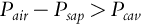
The cavitation pressure (Pcav) required to displace an air-water meniscus from a pit membrane pore in a xylem conduit can be calculated as
Here σ (N m− 1) represents the surface tension of water, θ (in degrees) is the angle at which the meniscus contacts the wall, and Dpore (m) is the diameter of the pit membrane pore (note that N m− 2 = Pa) (Oertli, 1971; Pickard, 1981; Tyree and Zimmermann, 2002; Michaletz et al., 2012).
From Eq. (11.6), it is clear that cavitation may occur if heating causes the air pressure (Pair) to increase, the sap pressure (Psap) to decrease, and/or the pressure of cavitation (Pcav) to decrease (Michaletz et al., 2012; West et al., 2016). Michaletz et al. (2012) suggested that heating has little impact on Pair, but likely affects Psap and Pcav. In particular, they showed that cavitation of xylem during a fire may occur due to a temperature-dependent reduction in the water surface tension (σ), thereby reducing the pressure required for cavitation.
Reduced xylem hydraulic conductivity due to conduit wall deformation
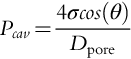
In addition to reducing the hydraulic conductivity via conduit embolism, fires can also cause structural damage to the xylem conduit walls (Michaletz et al., 2012). Conduit walls are composed of lignin, hemicellulose, and cellulose, which are viscoelastic polymers that have properties of both elastic solids and viscous fluids (Wolcott et al., 1990). At low temperatures they are hard and glassy, and at high temperatures they are soft and gel-like (Goring, 1965; Wolcott et al., 1990). The temperature at which a viscoelastic polymer starts to soften and act like a viscous liquid is known as the “glass transition point.” The glass transition point occurs between 60 °C and 90 °C for lignin and at approximately 50 °C for hemicellulose (Hillis and Rozsa, 1985; Olsson and Salmén, 1997), although the exact temperature varies with moisture content (Goring, 1965). When xylem is heated, the conduit wall polymers may transition from hard and glassy to soft and gel-like. Stresses imposed on conduit walls by tensile sap (Hacke et al., 2001) may then cause the softened walls to deform, collapse, and/or rupture, reducing the hydraulic conductivity of the conduit or preventing flow altogether. Changes in xylem structure can irreversibly reduce sap flow, as well as render pit membranes more susceptible to air seed cavitation (Fig. 11.9) (Bär et al., 2019). Indeed, heating has been shown to cause xylem collapse that was associated with irreversible declines in air permeability (Michaletz et al., 2012). Furthermore, when the xylem cools and the viscoelastic polymers return to a glassy state, these deformations will become permanent (Fig. 11.9).
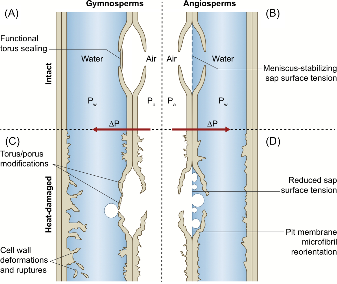
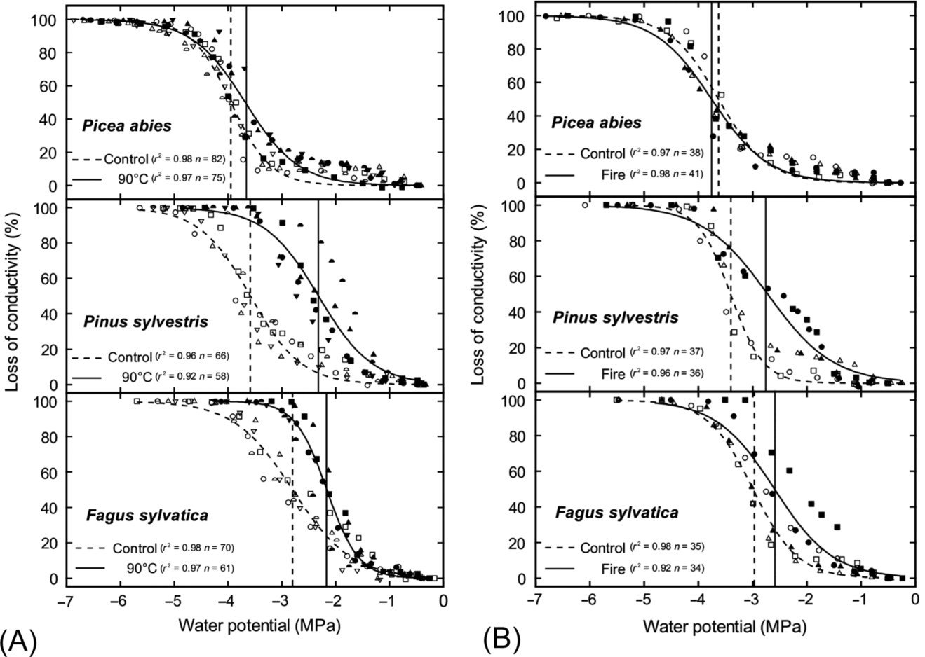
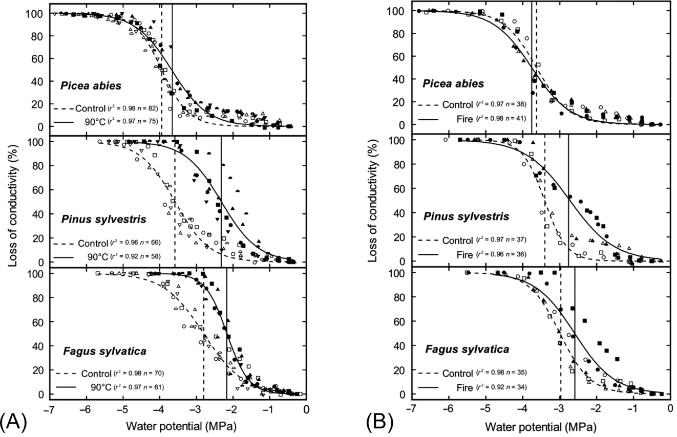
Although heating has caused xylem deformation in some species, in others the same treatment had little to no effect (Michaletz et al., 2012; Battipaglia et al., 2016; West et al., 2016; Bär et al., 2018). For example, Kiggelaria africana and Eucalyptus cladocalyx stems were heat treated in water baths at 70 °C and 100 °C. When examined with microscopy, K. africana showed xylem deformation and had reduced xylem conductivity, but no such deformation or loss of conductivity was observed for E. cladocalyx (West et al., 2016). Similarly, Bär et al. (2018) subjected three species of European trees to heating at 95 °C; although all species experienced xylem deformation, the degree to which this altered conductivity varied between species, with Fagus sylvatica and Pinus sylvestris exhibiting the largest declines in hydraulic conductivity and Picea abies the least (Fig. 11.10A). These results were also confirmed by measuring loss of conductivity in branches that had experienced a fire a year before (Fig. 11.10B). Clearly, species differ in their susceptibility to heating, with some species being more vulnerable to xylem deformation than others (Fig. 11.9). Bär et al. (2018) suggested that these effects may differ between angiosperms and gymnosperms. Angiosperms and gymnosperms may differ in the composition of the cell wall polymers, so that the glass transition point may be reached at different temperatures, or the structure or shape of the cell wall in gymnosperms may make them less susceptible to torsional strain, reducing their susceptibility to heating. Angiosperms and gymnosperms also differ in the anatomy of their pit membranes (Fig. 11.9). Heating of the hemicellulose and lignin polymers around the pit membrane may allow movement of cellulose microfibrils, potentially increasing or distorting the diameter of the pit pores (Michaletz, 2018; O'Brien et al., 2018; Bär et al., 2019). This would alter the cavitation pressure (Eq. 11.7), but the air permeability of pit membranes might be lower in gymnosperms than in angiosperms due to the presence of the torus-margo (Fig. 11.9).
Stem heating models
As discussed earlier in this chapter, wildfires generally cause uneven heating around the circumference of plant stems. This is a result of wind-driven vortices in the wake flow of the stem, which induce standing flames and longer residence times on the leeward side of the stem (Fig. 11.7). Uneven heating can result in phloem and cambium necrosis around part of the stem (fire scars), or can cause localized xylem dysfunction. Predicting these effects is important for understanding fire effects on plant functioning, growth, and mortality.
One of the first models to account for uneven heating of stems was Costa et al. (1991). These authors numerically calculated conduction heat transfer at discrete polar coordinates around the stem circumference. More recently, Chatziefstratiou et al. (2013) advanced a two-dimensional stem heating model (FireStem2D), which was an extension of the earlier FireStem model of Jones et al. (2004, 2006). FireStem2D divides the stem into cylindrical coordinates, and uses surface heat flux time series as forcing data for conduction heat transfer into the stem. The temperature at a given point in the stem depends on its depth and circumferential position, as well as on traits such as the thermal conductivity, thickness, water content, and density of bark and wood. Overall, FireStem2D accurately predicts temporal variation in stem heating, the temperature peak, and necrotic depth, but slightly overestimates the temperature inside the stem (Chatziefstratiou et al., 2013). Nevertheless, due to the ability to measure heating at different locations and depths in the stem, FireStem2D is amenable to modeling temperature profiles within the cambium and xylem. One caveat of the model is that because it is two-dimensional, it does not take into account the vertical movement of water and heat in the stem, and this may be the reason why stem temperature is overestimated (Chatziefstratiou et al., 2013; Wei et al., 2019). Another, larger challenge for using stem heating models to predict whole-plant effects is that they do not consider injuries in other parts of the plant. Accounting for injuries to the roots, stem, and canopy, and how they interact to influence whole-plant functioning, are important next steps for fire effects models.
Fire effects on crowns
Fire causes necrosis of foliage, branches, and buds predominantly through the convection of hot gasses in the fire plume (Van Wagner, 1973). Fire intensity, air temperature, and wind speed all impact the amount of convective heating a plant experiences (Van Wagner, 1973). However, traits such as crown shape, crown base height, surface area, orientation, and shielding from foliage can alter the transfer of heat to the leaves, buds, and branches in the crown (Michaletz and Johnson, 2006a,b). For example, foliage creates aerodynamic interference that consequently reduces the convective heat transfer between the plume and the leaves, branches, and buds (Michaletz and Johnson, 2006b; Pickett et al., 2009). If heating kills all of the foliage in a crown, plants may recover by resprouting from buds, making the study of bud necrosis important for predicting plant mortality. Bud traits such as size and position in the crown influence their resistance to convective heat transfer (Clarke et al., 2013; Hood et al., 2018). For example, ponderosa pine and longleaf pine, species with larger buds, are less susceptible to bud necrosis than sugar maple and American beech, species with smaller buds (Michaletz and Johnson, 2006a).
Crown heating models
Process models of canopy injury began with Van Wagner (1973) who used a buoyant plume model to estimate the air temperature profile above a fireline. The model assumed that plume thickness increases and temperature decreases with height above the flame, and that foliage temperature equals plume temperature, such that the crown scorch height will scale with the 2/3 power of fireline intensity. Van Wagner's (1973) model was semimechanistic, but ultimately used an empirical proportionality factor (k) obtained via regression to account for the convection transfer into the crown components. Building on this work, Michaletz and Johnson (2006b) derived k from first principles, showing how it is derived from heat transfer theory and the traits of crown components. Recognizing that k should vary across crown components (branches, buds, and leaves), as well as across studies, Michaletz and Johnson (2006b) linked buoyant plume theory with lumped capacitance heat transfer theory to generalize energy transfer into canopy components. This model equated the rate of heat accumulation in the mass of canopy components with the rate of surface heating via convection and radiation, and accurately predicted time to bud necrosis and scorch height of foliage. However, the Michaletz and Johnson (2006b) model is only applicable to thermally thin objects with a Biot number Bi ≤ 0.1 (i.e., crown components ≤ 1 cm in diameter).
Larger canopy components such as cones or thick branches are not thermally thin, but can instead have internal temperature gradients. The Michaletz and Johnson (2006b) model would not be appropriate in these cases. For larger crown components, a one-dimensional heat conduction model is more appropriate. Both Mercer et al. (1994) and Michaletz et al. (2013) used one-dimensional conduction models to examine the vulnerability of aerial seed banks to heating by fire. Both models assumed that heating was uniform around the cone circumference, because cones are small and have negligible impacts on air flow patterns. Michaletz et al.’s (2013) study, however, was exemplary because they implemented the one-dimensional cone heating model in a three-dimensional computational fluid dynamics (CFD) model of fire spread (Mell et al., 2009; Sullivan, 2009; Bakhshaii and Johnson, 2019). This represents an advance over the more commonly used buoyant plume theory because while buoyant plume theory is easy to use, it: (1) time-averages temperatures, (2) models fire spread through simple flame residence time arguments, (3) does not consider combustion processes, and (4) either neglects wind or considers it in only a rudimentary fashion. These limitations mean that buoyant plume theory cannot account for tree crown combustion or uneven heating around the tree driven by flame-wake interactions, which can have important implications for fire effects on crowns. For example, Splawinski et al. (2019) showed that seed survival varied between windward and leeward sides of the crown, and depended on crown height, horizontal distance from the tree bole (i.e. crown depth), and angle in relation to wind direction.
Linking stem and crown injuries to whole plant functioning
Predicting post-fire tree mortality is an important challenge for ecologists and global change biologists. Most post-fire mortality models use statistical correlations between the probability of tree death and variables related to fire behavior and effects, such as fire intensity, fuel consumption, crown scorch, and bark char (reviewed in Woolley et al., 2012). These models are easy to implement, but do not consider the underlying causes of mortality, and are case specific so that every situation requires a different model (Dickinson and Johnson, 2001; Michaletz and Johnson, 2008). Process-based models, such as those described above in this chapter, can also be used to predict tree mortality. These models are general, although different parameter values are needed for different species. Such models have typically focused on only a single part of the plant (i.e., injury to the crown or cambium) (e.g., Dickinson and Johnson, 2004; Jones et al., 2004; Michaletz and Johnson, 2006b) with a few exceptions that have considered injuries to more than one part of the plant (e.g., Peterson and Ryan, 1986; Michaletz and Johnson, 2008). With these process-based models, tree death is assumed if injury is extensive (e.g., 100% vegetative bud necrosis or entire stem girdling) (Michaletz and Johnson, 2008). However, how injuries to multiple parts of the tree interact to influence post-fire plant functioning is not well understood (Michaletz and Johnson, 2007; Hood et al., 2018; O'Brien et al., 2018). One suggestion on how to make models more general, and gain a better understanding of fire effects on plant functioning is to consider fire effects on carbon and water budgets (Michaletz, 2018; Bär et al., 2019) through, for example, a mass balance approach or optimization of carbon and water (e.g., Trugman et al., 2018). These approaches are appropriate because injuries to the roots, stems, and/or crown will alter the acquisition and transport of both carbon and water (Hood et al., 2018), which in turn will influence plant recovery and growth. For example, stem heating may injure the phloem, cambium, and xylem, thereby interfering with the transport of nonstructural carbohydrates to the roots and water and nutrients to the crown. Likewise, necrosis of foliage and buds will reduce photosynthesis and also cause a drain on nonstructural carbohydrates to rebuild lost foliage. Overall, multiple injuries will result in tree death when the acquisition of carbon and water is insufficient to meet requirements for growth and recovery over the long term.
Trugman et al. (2018) investigated post-drought tree mortality by modeling carbon gain after damage to the xylem. The model calculated whole-plant photosynthesis as a function of environmental conditions (e.g., vapor pressure deficit, soil water potential, and concentration of atmospheric CO2) and plant traits (e.g., leaf area, tree size, xylem area, etc.). Carbon available for maintenance, growth, and repair was then estimated as that gained from photosynthesis and that taken out of carbon stores. If carbon gained from photosynthesis was less than that needed to meet the tree's physiological requirements, carbon stores were used and reduced. If carbon stores reached 10% of the original value, the tree was assumed to die as a result of starvation. Through this model, Trugman et al. (2018) showed that trees aim to achieve an optimal ratio between xylem to leaf and fine root biomass due to a balance between the cost of tissue respiration and carbon gain and water loss from photosynthesis. Overall, when xylem was damaged, trees were found to shed leaves to maintain the optimal ratio between xylem and leaf biomass, a phenomenon observed with both drought and fire damaged trees (Balfour and Midgley, 2006; Carnicer et al., 2011; Midgley et al., 2011).
Trugman et al.'s (2018) approach could easily be adapted to investigate post-fire mortality. One could start by linking a CFD model of forest fire spread to heat transfer models that predict heat injury to tree stems (sapwood conduit cavitation and sapwood conduit collapse) and crowns (foliage necrosis). Stem and crown injuries could then be fed into Trugman et al.'s (2018) model and changes in the carbon stores could be modeled over time to predict post-fire tree recovery or mortality. Alternatively to Trugman et al.’s (2018) model, a mechanistic transport-resistance approach to carbon and nitrogen substrate allocation (cf. Thornley, 1998; Landsberg and Sands, 2011) and a simple pipe model approach to water relations (Shinozaki et al., 1964) could be used to link stem and crown injuries to a mass balance model of tree growth and mortality. Overall, these models could be used to predict tree survival or mortality at the individual level.
Scaling fire effects from individuals to ecosystems
Climate change is leading to changes in wildfire activity in ecosystems across the world. For example, temperate and high-latitude ecosystems, such as western North America, are experiencing larger, more intense wildfires with longer fire seasons due to increasing temperatures (Williams et al., 2019). These changes in fire frequency and intensity may lead to changes in the composition of plant communities. For example, areas that traditionally experienced frequent, low-to-moderate intensity fires but that now experience high intensity fires might suffer from reduced in situ propagule sources due to the death of a large number of trees (Stephens et al., 2013). These kinds of changes have already been observed (e.g., Stevens-Rumann et al., 2018), but most current modeling frameworks are retrospective and correlative, and are thus unable to accurately predict these changes. A more process-based framework, modeling physiological effects of fire on individual plants and then “scaling up” to investigate ecosystem levels, may be a more productive avenue of research. There are two approaches that can be used to scale fire effects from individuals to ecosystems: (1) spatially-explicit individual-based simulations or (2) metabolic scaling theory (MST).
Spatially-explicit individual-based simulations
Spatially-explicit, individual-based simulations would require knowledge of the size and identity of each tree in the area of interest. Then, following methods outlined in the section above (Linking plant injuries to whole plant functioning), one could model post-fire recovery or mortality for each tree. In this way, a spatially-explicit, individual-based model could link the causal processes of fire behavior, whole-tree physiology, tree growth, tree mortality, and forest community dynamics, which could replace empirical content in forest gap models. This method could be very useful to land managers interested in managing specific parcels of land with known size frequency distributions.
Metabolic scaling theory (MST)
MST uses scaling relationships between (for example) the abundance and size distribution of the individuals in a given area to calculate ecosystem stocks and fluxes such as total biomass, primary productivity, or other processes of interest (West et al., 2009; Enquist et al., 2009, 2015). It codifies how the total ecosystem phytomass can be quantified in terms of the average size-dependent plant mass and the stand size distribution. Specifically, MST predicts that the total biomass Mtot (kg) of a stand depends on the size distribution of the stand, which can be formalized as
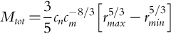
where cn (dimensionless) is the number of individuals of a particular size class, cm (m kg-3/8) relates stem radius (size class) to plant mass through a normalization constant, and rmax and rmin (m) are the stem radii of the largest and smallest individuals respectively. MST predicts that the total ecosystem phytomass increases with the 5/3 power of the largest stem radius and decreases with the 5/3 power of the smallest stem radius. Similar equations can be used to extend the theory to quantify ecosystem fluxes such as primary productivity, total metabolic rate, evapotranspiration, or even total nitrogen or water use of the stand (see Enquist et al., 2016 and McDowell et al., 2018 for more details). An extension of MST to predicting size-dependent effects of fire was outlined in McDowell et al. (2018) and we introduce the general approach here.
Post-fire tree mortality is a size-dependent phenomenon. Specifically, tree mortality is negatively related to tree size, with small trees generally dying before large trees (Michaletz and Johnson, 2008; McDowell et al., 2018). This is because small trees have thinner bark (Dickinson, 2002; Brando et al., 2012) and lower crowns, and are therefore more susceptible to heat transfer injuries such as phloem and cambium necrosis, xylem dysfunction, and crown component necrosis. Changes in the size distribution of individuals within a community will alter ecosystem stocks and fluxes and may be formalized by MST. McDowell et al. (2018) suggested that process-based models of fire injury (such as those outlined in this chapter) can be used to predict the radius of the smallest stem that will survive a fire, and outline how this is then linked with MST to “scale up” size-dependent mortality to predict changes in ecosystem biomass, productivity, and evapotranspiration.
Specifically, McDowell et al. (2018) used the one-dimensional conduction model of Michaletz and Johnson (2008) to predict the smallest stem radius (rmin) (m) that will survive a fire as a result of vascular cambium necrosis. This stem radius is given by
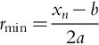
where a is the slope and b is the intercept from linear bark thickness allometries. The depth of tissue necrosis xn (m) is calculated analytically following Fourier's law of conduction, such that
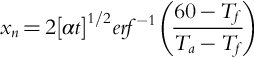
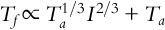
Here α is the thermal diffusivity of the bark (m2 s− 1), t is the fire residence time (s), Ta is the air temperature (°C), Tf is the fire temperature (°C), and 60 is the temperature (°C) at which tissue necrosis is assumed to occur. The temperature of the fire (Tf) is related to the air temperature (Ta) and the fire intensity (I; kW m− 1) as follows:
If one knows the size distribution of the community before a fire and how the size distribution will change after a fire (from Eq. 11.9), one can then calculate the biomass or productivity of the stand both before and after a fire.
The theory outlined in McDowell et al. (2018) predicts that increases in fire frequency will result in a reduction in recruitment of small size classes which, as size class distributions shift up over time, will result in a reduction in the number of individuals in larger size classes and ultimately lead to reduced ecosystem stocks and fluxes. These changes in the community size distribution could be modeled with size structured population models to model growth recruitment and mortality of the stand over time, but the MST approach is more general than individual based simulations and may be more appropriate for modeling ecosystem change at larger scales.
Conclusion
In this chapter we have outlined a process-based approach for predicting tree injury and mortality from wildfire. The approach begins by suggesting that fire behavior can be modeled using three-dimensional CFD models such as FIRETEC and WFDS versus older approaches such as buoyant plume models. Modern techniques in modeling fire behavior allow the prediction of combustion, fluid dynamics, and heat fluxes at the small spatial scales that are relevant for fire effects at the plant stem and canopy level. These heat fluxes can then be combined with process-based models of tissue necrosis to predict the depth and degree of tissue necrosis. If possible, process-based models should include injury to multiple plant parts (e.g., roots, stem, and crown), because it is the interaction of these injuries via whole-plant water and carbon budgets that govern post-fire plant functioning and mortality. Thus, predictions of plant mortality as a result of organ injury could be predicted through models that examine changes in carbon and water uptake, transport, and budgets. Lastly, our method can be used to predict how wildfire will result in ecosystem change by either performing spatially-explicit individual-based simulations of tree mortality across a stand that burns or through metabolic scaling theory that could be used to predict changes in ecosystem stocks and fluxes.